Spectral interpolation on a grid

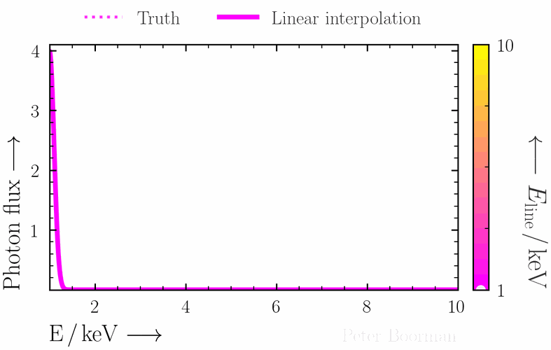
When table models are used in X-ray spectral fitting, the table is a collection of spectra on a multi-dimensional parameter grid. It is useful to interpolate between parameter grid points when performing parameter estimation during a fit, but this can cause interpolation effects. In this figure, a Gaussian table model has been created with integer values of line energies. As the line energy is changed, the true value (using the gauss model in Xspec) is shown with a dotted line, and the interpolated version from the table model approximation with a solid line. The biggest difference between the truth and interpolated values are seen when the line energy is directly in-between two tabulated grid points.

Black hole spins with Athena/X-IFU

In this figure, a series of AGN X-ray spectra are simulated with Athena/X-IFU at incrementally brighter fluxes. The right panel shows the posterior points found for black hole spin vs. the height of the X-ray emitting source above the black hole (assuming the lamp post geometry). For low, intermediate and high spins, the X-IFU can constrain spin under the assumptions of the simulated model.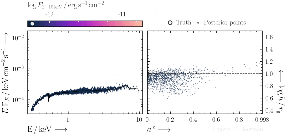

X-ray Spectral Fitting 2022

This is the more detailed version of the X-ray Spectral Fitting 2022 winter school logo, visualising the process of prior predictive checks with the MYtorus AGN obscurer model in a coupled configuration. By assuming a Gaussian prior on the log column density centered at 24.5 with standard deviation 0.1, a range of spectra are constructed. The gif then cycles through the simulated spectra in groups of 50, ordered and coloured by column density.

Variable obscuration

Here I use the UXCLUMPY model (Buchner et al., 2019) to plot the observed X-ray spectrum emerging from a clumpy distribution of gas clouds surrounding an accreting supermassive black hole. The app uses streamlit, plotly, pandas, matplotlib & numpy, and was featured in one of the Weekly Roundups on the Streamlit community forum. The app may take ~5-10 seconds to load - click here to view the app in a new tab.

Bayesian X-ray Analysis (BXA) GIF

This GIF shows a series of simulations of obscured AGN spectra at incrementally lower observed fluxes (whilst maintaining the same intrinsic luminosity and column density - see the dashed "truth" lines in the right panel). By simultaneously modelling the background and source spectra, BXA enables constraints from spectra with no net source counts. For example, at the lowest fluxes the source is not detected and any spectrum is background dominated. Since the background is being fit simultaneously to the source + background, the source cannot be brighter than this whilst being completely unobscured. This is why the upper left portion of the contour plot in the right panel is ruled out. Learn more about how to use BXA in the tutorial I wrote here.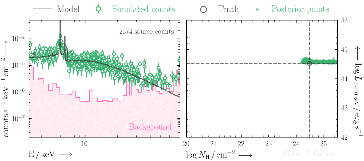

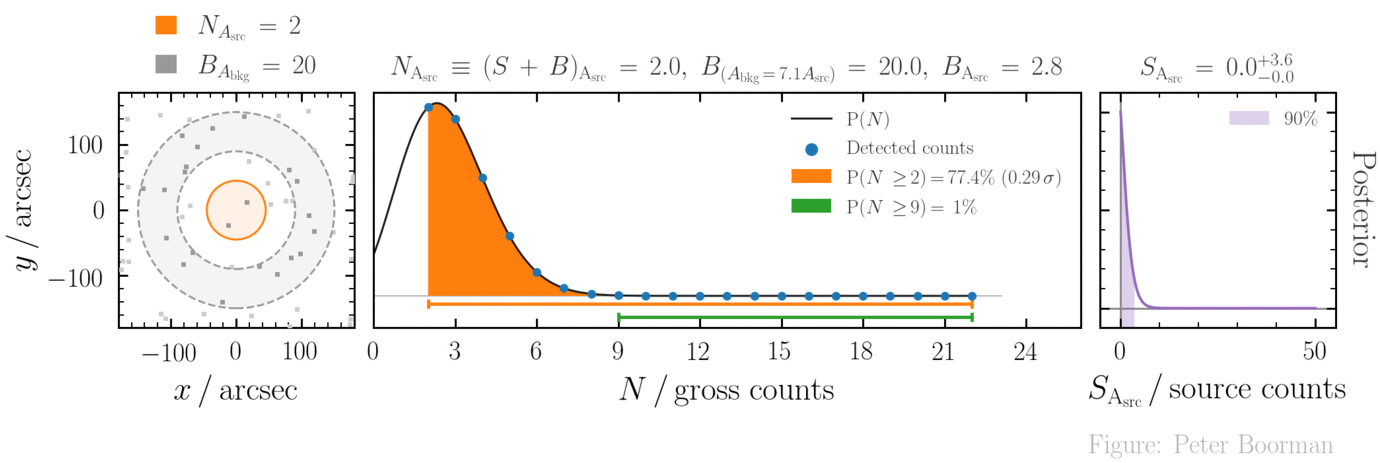
No-source probability GIF

No-source probabilities are used to quantify detection significance in X-ray astronomy, and is the probability that some amount of detected counts in a source region (N_Asrc) is caused by a background fluctuation (i.e. that there is "no source"). For more information, see discussion in Lansbury et al., (2014) or Weisskopf et al., (2007)

I created this GIF using code provided by George Lansbury to calculate no-source probabilities and estimate the posterior for the number of source counts. The left panel shows a simulated observation with the number of source+background counts consider in a given instance, as well as the number of background counts (fixed at 20 here). The middle panel shows the Binomial no-source probability distribution, with orange and green regions representing the no-source probabilities for the observation and for the number of counts required to reach a no-source probability of 1%. The right panel then shows the Bayesian posterior distribution on number of source counts using the formalism from Kraft et al., (1991).

AGN schematic

Inspired by the schematic depicted in Ramos-Almeida & Ricci (2017; NatAs-1-679), I produced this plot depicting a number of the significant emission regions of AGN on a logarithmic scale with matplotlib. This schematic was used in my Ph.D. thesis which was published in Springer Theses.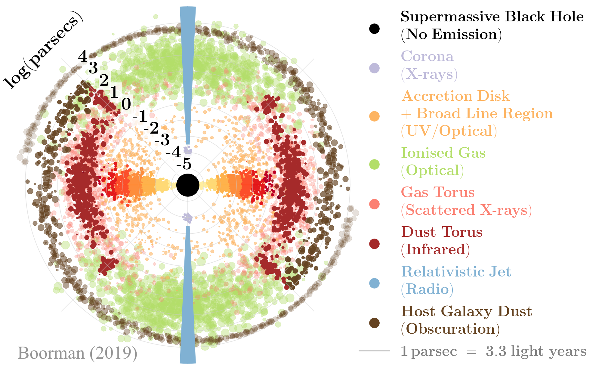

Circum-nuclear environment

X-rays come from a region extremely close to the accreting supermassive black hole in AGN, and can be scattered and absorbed by material in the circum-nuclear region (see left panel). In contrast, the dust surrounding the black hole acts as a bolometer which absorbs and re-radiates the accretion disc light into the infrared.

This can be seen in the right panel, showing several spectral energy distributions. The purple and salmon-coloured spectra on the left show the equivalent emission in X-rays that we would see for a face-on (i.e. unobscured) and edge-on (i.e. obscured) viewing angle, respectively. Clearly there's a significant flux suppression across the entire X-ray spectrum!
However, in the infrared (brown) part of the SED, the hatched region shows the difference in emission between face-on and edge-on geometries which is much smaller. This is a powerful concept - the mid-to-far infrared emission from AGN can be considered more isotropic, where isotropic here means the ability to detect unobscured and obscured AGN with approximately equal probability.

Interactive skymaps

Swift/Burst Alert Telescope 70-month catalogue

This is an interactive sky-map I created with the help of Adam Hill using Plotly. You can select the different redshift ranges in the legend to plot different selections on the skymap. Every source was detected in the 70 month Swift/Burst Alert Telescope catalogue, and the size of the points is proportional to the amount of hard X-ray (14-195 keV) flux detected by BAT at that position in the sky.

The NuSTAR Local AGN N_H Distribution Survey (NuLANDS)

This is an interactive sky-map of the NuSTAR Local AGN N_H Distribution Survey (NuLANDS) sample. Each point was selected based on their mid-to-far infrared flux detected by the InfraRed Astronomy Satellite (IRAS). NuLANDS was selected as an ~1 Ms Legacy Survey with NASA's NuSTAR space telescope to determine how obscured AGN are on average in the local Universe.

Cosmic backyard

The NED redshift-independent Distances catalogue (NED-D) is a comprehensive catalogue of extra-galactic sources for which astronomers have estimated the distance to using techniques that do not rely on a redshift. This is possible with e.g., standard candles (sources with a pre-defined luminosity) or standard rulers (sources with a pre-defined size) which can be used to estimate the distance. Plotted in supergalactic coordinates, this map shows the location of all sources in the NED-D catalogue within approximately 15 million light years from the Milky Way which is located at the center. I used the SVG file format with Beautiful Soup and matplotlib to enable a link to each source's NED page by clicking on individual points. Give it a go!.

AGN unification

The simplest form of the unified model of AGN (Antonucci 1993, Urry & Padovani 1995, Netzer 2015) ascribes different AGN classes to the orientation of some form of circum-nuclear obscurer relative to the line of sight. Originally, Type 1 (face-on, unobscured) and Type 2(edge-on, obscured) AGN were classified by their different optical spectra showing broad permitted and/or narrow forbidden lines, respectively. Since the original identification of Type 1 and 2 AGN, a number of different optical spectroscopic types have been identified, which I show in this plot.

Obscured AGN X-ray spectra

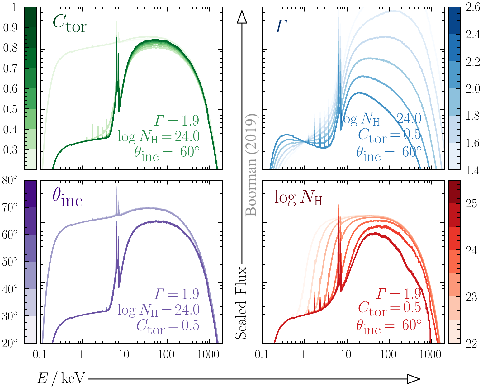
X-ray photons can be absorbed and scattered by atoms in the vicinity of an accreting supermassive black hole. We know that a majority of all AGN are obscured in some form across cosmic time, but a large ongoing question is the geometry of that obscuration. One way to predict the X-ray emission emerging from the dense obscuration surrounding AGN is with Monte Carlo Radiative Transfer. Billions of X-ray photons are simulated and fired through some unique geometry of gas clouds, before the emerging photons are counted and presented as unique X-ray spectra. This plot shows the result of several such simulations with the borus02 uniform density torus model. The gas is assumed to be spherical and covering the central AGN, with polar cut-outs of variable size enabling the user to vary the covering factor of the obscuring gas (i.e. the amount of the sky that is obscured if one were to sit on top of the AGN and stare outwards). Each panel shows the effect of varying a different parameter: (upper left) covering factor, (upper right) incident X-ray spectrum photon index, (lower left) observer inclination and (lower right) line-of-sight obscuring equivalent hydrogen colulmn density.