Welcome to the Bayesian X-ray Analysis (BXA) tutorial page.
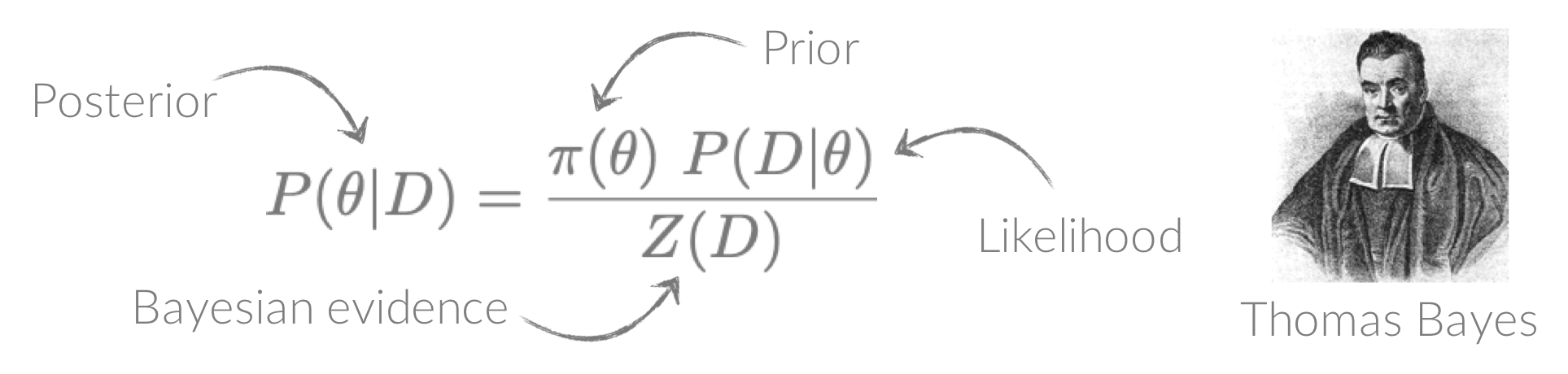
BXA connects PyXspec/Sherpa to nested sampling algorithms for Bayesian parameter estimation and model comparison with the Bayesian evidence. See the Why use BXA? page for a few of the many reasons BXA can be useful for X-ray spectral fitting!
Setup
The setup page contains:- Information/links for installing PyXspec and/or Sherpa
- Step-by-step to install BXA
- Download links for the data used in the exercises
Session 0 - X-ray spectral fitting
This session aims to provide a sufficient background with Xspec/PyXspec and/or Sherpa to complete the remaining BXA tutorial exercises. For a complete and in-depth understanding of the features available in these software packages, see the useful links for the excellent online material provided by each team. Key objectives:- Load a spectrum and fit a model to it in Xspec, PyXspec and/or Sherpa
- Manually explore a parameter space and avoid local minima
- Get to grips with plotting in Xspec, PyXspec and Sherpa
Session 1 - using BXA
This session introduces how to construct a BXA fit to spectra in a variety of different setups.Key objectives:
- Fit a spectrum with BXA in Sherpa and/or PyXspec
- Interact with posteriors
- Fit more than one spectrum simultaneously with BXA
Session 2 - model checking
After fitting a model to the data, how can you check the quality of the fit? This session delves into a variety of ways to examine your fits and check that the model is able to explain the data to a satisfactory level. Key objectives:- Learn how to plot the posterior model with the data
- Visualise goodness-of-fit without requiring the data to be re-binned
- Compare predicted model counts to observed counts to estimate goodness-of-fit
Session 3 - model comparison
Rather than considering models in isolation, how do different models' fits to the same data compare? This sessions considers ways to quantify a model fit relative to others. Key objectives:- Use the Bayesian evidence to perform model comparison
- Quantify how often the more complex model selected incorrectly
- Quantify how often the simpler model selected incorrectly
Session 4 - parent distributions
When constraining a parameter for a sample of sources, it can be useful to determine what parent model could have generated the parameter posteriors you have constrained. This session uses Hierarchical Bayesian modelling to do this. Key objectives:- Understand the concept of parent distributions
- Combine individual posteriors to constrain a parent distribution
- Constrain a variety of parent distribution models for a given set of posteriors
Session 5 - more advanced concepts
What else can you do with BXA? Check out this session to see some other interesting applications. Key objectives:- Quantify the gain in information acquired on a parameter after fitting
- Include custom priors in BXA fits
- Speed up BXA runtimes with step samplers
Tips & tricks
Interested in some handy features in BXA? Check out this page to see:- Fitting 2D models to images
- Using a BXA
solverobject with other fitting packages - Plotting packages for producing corner plots & posterior distributions
- Many more!
Useful links
Check out this page for a living list of useful resources for astrostatistics and X-ray spectral fitting, including:- Documentation
- Places to ask questions
- Useful papers & documents
- Lectures & videos
- Scripts
- Useful citations