Rather than considering models in isolation, how do different models' fits to the same data compare? This session considers ways to quantify the quality of a model fit relative to others.
Key objectives:
- Use the Bayesian evidence to perform model comparison
- Quantify how often the more complex model could be selected incorrectly
- Quantify how often the simpler model could be selected incorrectly
Exercise 3.1 - Bayes factors
Here we use the Bayesian evidence to perform model comparison with Bayes factors.- Copy the model_compare.py script to your working directory to perform Bayesian evidence model comparison
- Run the script:
$ python3 model_compare.py outputfiles_basename1/ outputfiles_basename2/ outputfiles_basename3/ - Which model is preferred by the Bayes factors? Try changing the
limitvalue in model_compare.py from 30 to 100. Has the preferred model order changed? Why or why not? - Temporarily try including a
cabscomponent inmodel3:
- PyXspec:
model4 = Model("TBabs*zTBabs*cabs(zpowerlw+zgauss)")
model4.TBabs.nH.values = (0.04, -1.) ## Milky Way absorption
model4.zTBabs.Redshift.values = (0.05, -1.)
model4.zTBabs.nH.values = (1., 0.01, 0.01, 0.01, 100., 100.)
model4.cabs.nH.link = "p%d" %(model4.zTBabs.nH.index)
model4.zpowerlw.PhoIndex = (1.8, 0.1, -3., -2., 9., 10.)
model4.zpowerlw.Redshift.link = "p%d" %(model4.zTBabs.Redshift.index)
model4.zpowerlw.norm = (1.e-4, 0.01, 1.e-10, 1.e-10, 1., 1.)
model4.zgauss.LineE.values = (6.4, 0.1, 6., 6., 7.2, 7.2)
model4.zgauss.Sigma.values = (1.e-3, 0.01, 1.e-3, 1.e-3, 1., 1.)
model4.zgauss.Redshift.link = "p%d" %(model4.zTBabs.Redshift.index)
model4.zgauss.norm.values = (1.e-5, 0.01, 1.e-10, 1.e-10, 1., 1.)
- PyXspec:
- How does the Bayesian Evidence from fitting the new
model4to the data compare to the previous models?
Exercise 3.2 - type I errors
How can we know what Bayes factor threshold to use? Simulations! Here we will calculate the false-positive rate associated with our data and models to tell us how often a more complex model is selected when the simpler model was actually correct.
- First we will consider the false-positive rate between the simpler
model1and more complexmodel2models. - Simulate 100 NuSTAR spectra from the best-fit
model1spectrum using the original spectral files in each simulation and bin the simulated spectra in the same manner as the original data. - Using BXA, fit both
model1andmodel2to each of the 100 simulated spectra. Make sure to have uniqueoutputfiles_basenamevalues! - On each iteration, save the
logZvalues:results = solver.run(resume=True) logZ = results["logZ"]
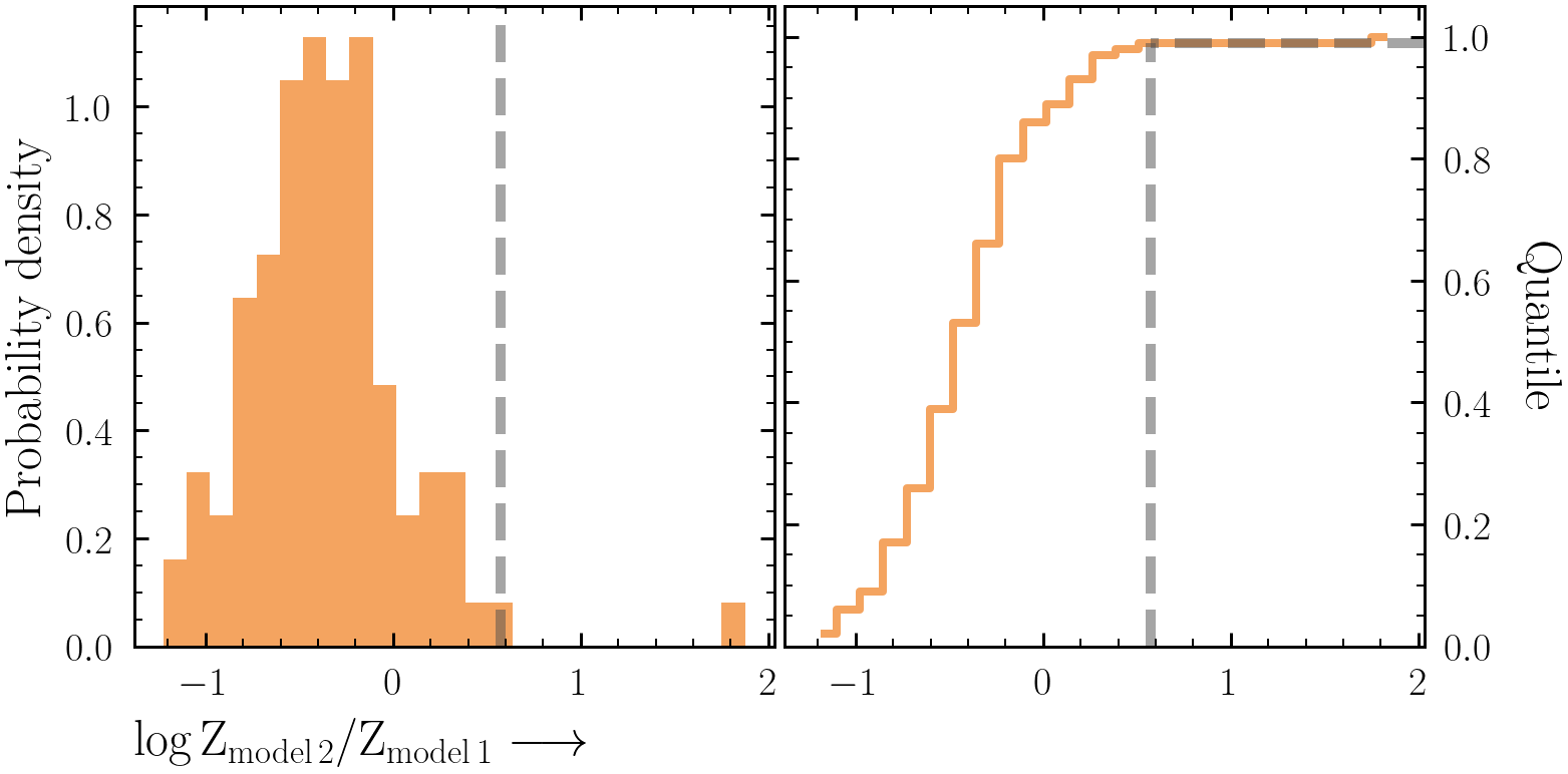
- Use your two distributions of
logZ(one distribution for fittingmodel1-simulated data withmodel1, the other from fitting withmodel2) to produce a Bayes factor distribution. - What Bayes factor threshold is needed to achieve a false-positive rate of 1% or less?
-
Perform the above exercises for
model2vs.model3andmodel1vs.model3. Are all the Bayes factor thresholds for a <1% false-positive rate similar between different models? Why or why not?
Exercise 3.3 - type II errors
Here we will calculate the false-negative rate associated with our data and models to tell us how often a less complex model is selected when the more complex model was actually correct.
- First we will consider the false-negative rate between the more complex
model2and simplermodel1models. - Simulate 100 NuSTAR spectra from the best-fit
model2spectrum using the original spectral files in each simulation and bin the simulated spectra in the same manner as the original data. - Using BXA, fit both
model1andmodel2to each of the 100 simulated spectra. Make sure to have uniqueoutputfiles_basenamevalues! - On each iteration, save the
logZvalues:results = solver.run(resume=True) logZ = results["logZ"]
- Use your two distributions of
logZ(one distribution for fittingmodel2-simulated data withmodel1, the other from fitting withmodel2) to produce a Bayes factor distribution. - What Bayes factor threshold is needed to achieve a false-negative rate of 1% or less?
-
Perform the above exercises for
model3vs.model2andmodel3vs.model1. Are all the Bayes factor thresholds for a <1% false-negative rate similar between different models? Why or why not?
Estimating the false positive and negative rates is not only useful for BXA. The process of null hypothesis significance testing is useful to any form of fitting. Here we will apply the same process from Exercises 3.2 and 3.3 to other model comparison techniques.
- From each simulated model best-fit in Exercises 3.2 and 3.3, save the fit statistic (
fitstat) on each iteration. Calculate aΔfitstatdistribution by subtracting bothfitstatvalues per simulated spectrum. WhatΔfitstatvalue is required for type I and II errors of less than 1%? - Compute the Akaike Information Criterion (AIC) (given by
AIC = 2×nfree+Cstat ≡ 2×nfree-2×log(Likelihood), wherenfreeis the number of free fit parameters) for each model in python:import json basenames = [outputfiles_basename1, outputfiles_basename2, outputfiles_basename3] loglikes = dict([(f, json.load(open(f + "/info/results.json"))["maximum_likelihood"]["logl"]) for f in basenames]) nfree = dict([(f, len(json.load(open(f + "/info/results.json"))["paramnames"])) for f in basenames]) aic = dict([(basename, (2. * nfree[basename] - 2. * loglike)) for basename, loglike in loglikes.items()])
- What ΔAIC value is required for type I and II errors of less than 1%?
- Do the observed distributions for estimating type I and II errors change when considering
model2andmodel3?