This session introduces how to construct a BXA fit to spectra in a variety of different setups.
To start with, make sure you import the relevant packages:
Key objectives:
- Fit a spectrum with BXA in Sherpa and/or PyXspec
- Interact with posteriors
- Fit more than one spectrum simultaneously with BXA
To start with, make sure you import the relevant packages:
- PyXspec:
from xspec import *
import bxa.xspec as bxa
- Sherpa:
import bxa.sherpa as bxa
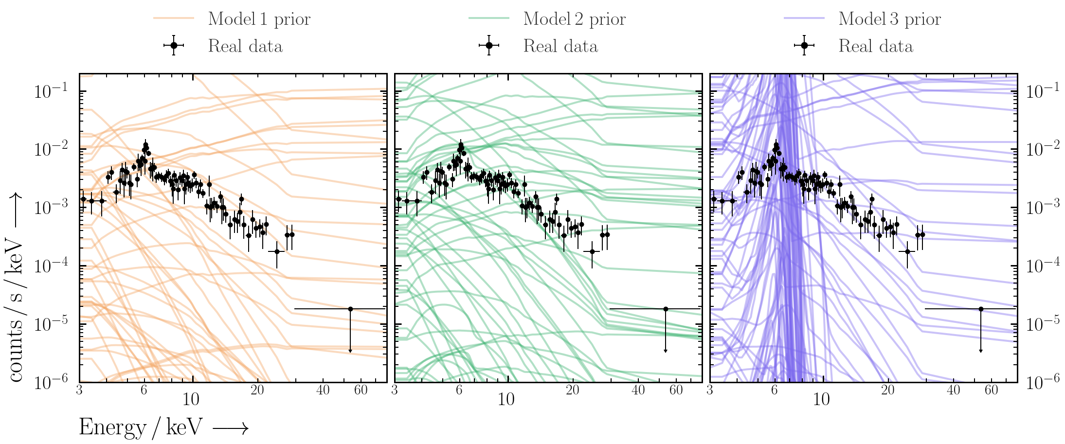
Exercise 1.1 - prior predictive checks
Prior predictive checks are used to see if the priors chosen can lead to realistic model realisations.
Note for these exercises, setting priors in BXA is done with the following commands:
- PyXspec:
bxa.create_uniform_prior_for(model, param)
bxa.create_loguniform_prior_for(model, param)
bxa.create_gaussian_prior_for(model, param, mean, std)
- Sherpa:
bxa.create_uniform_prior_for(param)
bxa.create_loguniform_prior_for(param)
bxa.create_gaussian_prior_for(param, mean, std)
model1 based on a powerlaw (see the commands in Exercise 0.1 for help). Note the target in question can be assumed to be at redshift 0.05 with a Galactic column density of NH = 4×1020 cm-2:
- PyXspec:
model1 = Model("TBabs*zpowerlw")
model1.TBabs.nH.values = (0.04, -1.) ## Milky Way absorption
model1.zpowerlw.PhoIndex = (1.8, 0.1, -3., -3., 10., 10.)
model1.zpowerlw.Redshift.values = (0.05, -1.)
model1.zpowerlw.norm.values = (1.e-4, 0.01, 1.e-10, 1.e-10, 1., 1.)
- Note to use
TBabs, one should set the abundances to those from Wilms, Allen & McCray (2000):- PyXspec:
Xset.abund = "wilm" - Sherpa:
set_xsabund("wilm")
- PyXspec:
- Set the parameter priors for
model1(notenormvaries over many orders of magnitude, andPhoIndexcan be assigned a uniform prior for now):- PyXspec:
prior1 = bxa.create_uniform_prior_for(model1, model1.zpowerlw.PhoIndex)
prior2 = bxa.create_loguniform_prior_for(model1, model1.zpowerlw.norm)
- Sherpa:
prior1 = bxa.create_uniform_prior_for(model1.PhoIndex)
prior2 = bxa.create_loguniform_prior_for(model1.norm)
- PyXspec:
- A note on log parameters (Sherpa only):
Using a loguniform prior may not give the posterior values of that parameter in log units in Sherpa.
Instead, the
Parametermodule can convert a parameter to log units, and then one can use a uniform prior for that parameter. E.g.:from sherpa.models.parameter import Parameter logpar = Parameter(modelname, parname, value, min, max, hard_min, hard_max) model1.norm = 10**logpar
Note the parameter will only be valid for working in BXA. If you want to define a log parameter and use this with a standard Sherpa fit, the log parameter must appear in the model expression.
- Create a solver:
- PyXspec:
solver = bxa.BXASolver(transformations=[prior1, prior2], outputfiles_basename="model1_nu") - Sherpa:
solver = bxa.BXASolver(prior=bxa.create_prior_function([prior1, prior2]),
                       parameters=[param1, param2],
                       outputfiles_basename="powerlaw_sherpa")
outputfiles_basenameis always unique. Especially if running PyXspec and Sherpa in the same directory.- (For Sherpa) the priors are in the same order for the
priorandparametersattributes.
- PyXspec:
- Perform prior predictive checks:
- Generate a random sample of prior parameter values (remember to
import numpy!): - Set the parameters to these values:
- PyXspec:
from bxa.xspec.solver import set_parameters
set_parameters(transformations=solver.transformations,values=values)
- Sherpa:
for i, p in enumerate(solver.parameters): p.val = values[i]
- PyXspec:
- Plot the resulting prior model realisation with the data:
- Repeat 100 times, and plot the prior realisations with the data. Are the model ranges covered by the priors physically-acceptable?
- Generate a random sample of prior parameter values (remember to
Now that we have checked the priors look reasonable for the data we want to fit, we can fit the model to the data with BXA and get parameter posteriors.
- First fit the model using Levenberg-Marquardt included in Xspec & Sherpa:
- Is the fit good? How can you tell? What does changing the parameters by a small amount do?
- Next perform the fit with BXA (note this does not require fitting with Levenberg-Marquardt first):
(Note the hyperlinks are different).
resultscontains the posterior samples (results["samples"]) for each parameter and the Bayesian evidence (results["logZ"],results["logZerr"]). These quantities should also be printed to the screen after the fit is completed. To understand more about the information UltraNest prints to the screen during and after a fit, see here. - Examine the best-fit values and uncertainties from the posterior samples. This can be done with
pandas(may require installing with e.g.,conda install pandasbut see warning at the end of Setup):import pandas as pd posterior_df = pd.DataFrame(data=results["samples"], columns=solver.paramnames) posterior_df.to_csv("%s/posterior.csv" %(outputfiles_basename), index=False)
- How do the best-fits and confidence ranges compare with using nested sampling vs. Levenberg-Marquardt?
- Finally, save the best-fit model (which is loaded as the current model by default with BXA) set-up to enable restoring it easily at later stages:
Xset.save("%s/model.xcm" %(outputfiles_basename))
Next fit an additional two models to the data (which are used in subsequent exercises). Make sure to perform prior predictive checks each time before fitting.
model2features the same powerlaw as inmodel1but with additional photo-electric absorption:- PyXspec:
model2 = Model("TBabs*zTBabs*(zpowerlw)")
model2.TBabs.nH.values = (0.04, -1.) ## Milky Way absorption
model2.zTBabs.Redshift.values = (0.05, -1.)
model2.zTBabs.nH.values = (1., 0.01, 0.01, 0.01, 100., 100.)
model2.zpowerlw.PhoIndex.values = (1.8, 0.1, -3., -3., 10., 10.)
model2.zpowerlw.Redshift.link = "p%d" %(model2.zTBabs.Redshift.index)
model2.zpowerlw.norm.values = (1.e-4, 0.01, 1.e-10, 1.e-10, 1., 1.)
model1with an additionalloguniformprior forzTBabs.nH.- PyXspec:
model3features the same absorbed powerlaw as inmodel2but with an additional Gaussian line:- PyXspec:
model3 = Model("TBabs*zTBabs*(zpowerlw+zgauss)")
model3.TBabs.nH.values = (0.04, -1.) ## Milky Way absorption
model3.zTBabs.Redshift.values = (0.05, -1.)
model3.zTBabs.nH.values = (1., 0.01, 0.01, 0.01, 100., 100.)
model3.zpowerlw.PhoIndex.values = (1.8, 0.1, -3., -3., 10., 10.)
model3.zpowerlw.Redshift.link = "p%d" %(model3.zTBabs.Redshift.index)
model3.zpowerlw.norm.values = (1.e-4, 0.01, 1.e-10, 1.e-10, 1., 1.)
model3.zgauss.LineE.values = (6.4, 0.1, 6., 6., 7.2, 7.2)
model3.zgauss.Sigma.values = (1.e-3, 0.01, 1.e-3, 1.e-3, 1., 1.)
model3.zgauss.Redshift.link = "p%d" %(model3.zTBabs.Redshift.index)
model3.zgauss.norm.values = (1.e-5, 0.01, 1.e-10, 1.e-10, 1., 1.)
zgauss.LineEand loguniform priors forzgauss.Sigmaandzgauss.norm.- PyXspec:
Exercise 1.4 - error propagation
By generating quantities directly from the posterior samples, we propagate the uncertainties and conserve any structure (e.g., degeneracies, multiple modes).
We will consider three examples for posterior-based error propagation. Note the example code uses a
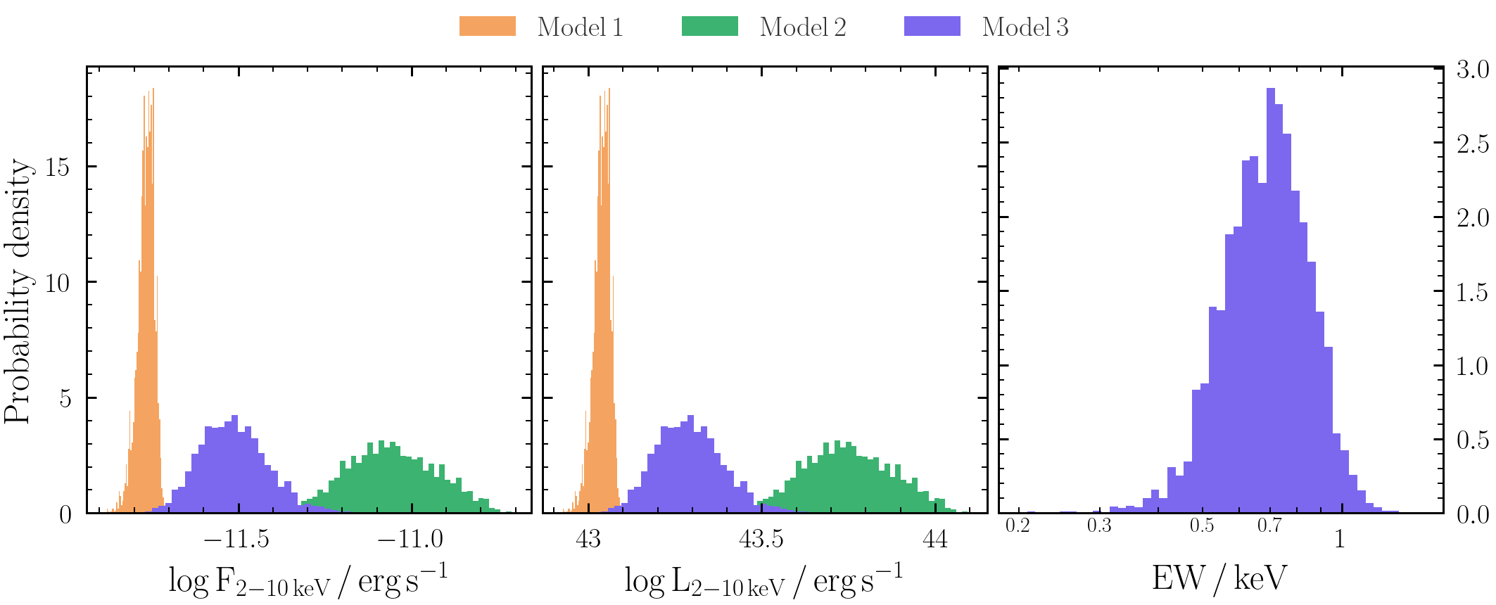
posterior_df pandas dataframe to propagate the uncertainties.
- Unabsorbed powerlaw flux: To calculate the flux of the powerlaw model component, we multiple by energy and integrate between
Emin_keV=2andEmax_keV=10. Make sure to convert the units of the powerlaw normalisation so we get flux in erg/s/cm2.## note have to be careful if PhoIndex ~ 2 if numpy.isclose(PhoIndex, 2., atol = 1.e-2): logflux = lognorm + numpy.log10(numpy.log(Emax_keV / Emin_keV)) else: A = 2. - PhoIndex logflux = lognorm + numpy.log10(((Emax_keV**A) - (Emin_keV**A)) / A)
- Unabsorbed powerlaw luminosity: Now we have the unabsorbed flux, and we know the source is at redshift 0.05 we can estimate the distance and thus the luminosity.
from tqdm import tqdm
z = 0.05
from astropy.cosmology import FlatLambdaCDM
chosen_cosmology = FlatLambdaCDM(H0=67.3, Om0=0.315)
D_cm = chosen_cosmology.luminosity_distance(z).value*(10**6)*(3.086*10**18)
tqdm.pandas(desc="Calculating logluminosity in the 2-10 keV band")
posterior_df.loc[:, "loglum"] = posterior_df["logflux"].progress_apply(lambda x: x + numpy.log10(4.*numpy.pi) + 2.*numpy.log10(D_cm))
- Unabsorbed equivalent width: The equivalent width (
EWbelow) of an emission line is defined as the flux in the line divided by the flux of the continuum at the line energy (see the Xspec documentation for more information). By considering just thezpowerlw>andzgausscomponents (i.e. no absorption), we get the unabsorbed equivalent width.EW_keV = ((10 ** lognorm_zgauss)/(10 ** lognorm_zpow))*(LineE**PhoIndex) / (1.+z)
- Are any of the secondary parameters you have derived degenerate with the original parameters?
- How do the unabsorbed flux and equivalent width posteriors compare between different models?
- Extension: load a fixed number of posterior model rows into Xspec and calculate the observed flux and equivalent widths. How do the observed (i.e. absorbed) model fluxes and equivalent width posteriors compare to the unabsorbed values derived above?
Exercise 1.5 - fitting multiple datasets simultaneously with BXA
Sometimes it is advantageous to fit multiple spectra for the same source simultaneously with a cross-calibration constant to account for instrumental differences associated with the separate spectra.
For this example, we need another dataset. As an example, we will use the Chandra/ACIS spectrum included in the downloadable files which will be fit in the energy range 0.5-8 keV to extend our spectral range to lower energies than attainable with just NuSTAR.
We first assume that the source was not variable between the NuSTAR and Chandra observations, and thus only account for differences arising from the calibration of either instrument with an additional factor pre-multiplying each spectrum.
- First, include a cross-calibration constant in your model between the Chandra and NuSTAR datasets:
- PyXspec:
AllData("1:1 nustar_src_bmin5.pha 2:2 chandra_src_bmin5.pi") AllData.ignore("1:0.-3. 78.-** 2:0.-0.5 8.-**") model1 = Model("constant*TBabs*zpowerlw") AllModels(1).constant.factor.values = (1., -1.) AllModels(1).TBabs.nH.values = (0.04, -1.) ## Milky Way absorption AllModels(1).zpowerlw.PhoIndex.values = (1.8, 0.1, -3., -2., 9., 10.) AllModels(1).zpowerlw.Redshift.values = (0.05, -1.) AllModels(1).zpowerlw.norm.values = (1.e-4, 0.01, 1.e-10, 1.e-10, 1., 1.) AllModels(2).constant.factor.values = (1., 0.01, 0.1, 0.1, 10., 10.) Plot("ldata") - Sherpa:
load_pha(1, "nustar_src_bmin5.pha")
ignore_id(1, "0.:3.,78.:")
load_pha(2, "chandra_src_bmin5.pi")
ignore_id(2, "0.:0.5,8.:")
model1 = xstbabs.tbabs*xspowerlaw.mypow
x1model1 = xsconstant("xcal1") * model1
set_par(xcal1.factor, val=1, frozen=True)
x2model2 = xsconstant("xcal2") * model1
set_par(xcal2.factor, val=1, min = 1.e-2, max = 1.e2)
set_source(1, x1model1)
set_source(2, x2model2)
- PyXspec:
- Fit the new model with BXA and derive a posterior confidence range on the cross-calibration constant. Remember to do prior predictive checks before fitting!
- PyXspec:
prior1 = bxa.create_uniform_prior_for(model1, model1.zpowerlw.PhoIndex)
prior2 = bxa.create_loguniform_prior_for(model1, model1.zpowerlw.norm)
prior3 = bxa.create_loguniform_prior_for(AllModels(2), AllModels(2)(1))
solver = bxa.BXASolver(transformations=[prior1, prior2, prior3], outputfiles_basename="model1_nuchan")
results = solver.run(resume=True)
- Sherpa:
prior1 = bxa.create_uniform_prior_for(model1, model1.zpowerlw.PhoIndex)
prior2 = bxa.(model1, model1.zpowerlw.norm)
prior3 = bxa.(xcal2)
priors = [prior1, prior2, prior3]
parameters = [model1.zpowerlw.PhoIndex, model1.zpowerlw.norm, xcal2]
solver = bxa.BXASolver(prior=bxa.create_prior_function(priors), parameters=parameters, outputfiles_basename="model1_nuchan")
results = solver.run(resume=True)
model3with both datasets simultaneously can take up to an hour. - PyXspec:
- How have the confidence ranges on all the model parameters changed after including Chandra?
- Have the uncertainties on unabsorbed flux or equivalent width changed?
Exercise 1.6 - automated background fitting with BXA
An alternative technique to W-statistics is to use C-statistics, which does not require any spectral binning so long as a viable background model exists. Here we explore how to implement background models within PyXspec and Sherpa.
So far the exercises have used modified C-statistics (aka W-statistics) in which the background is modelled as a stepwise function with the same number of parameters as bins. This process typically requires some form of minimal binning to avoid having too many background bins with zero counts (see discussion here).
Using C-statistics can be more flexible, since no binning is required by simultaneously fitting a background model with the source model instead. Here we use the PCA background models presented by Simmonds et al., 2018 together with the automated fitting procedure available as part of BXA. Note since the background models are empirical and are fit in detector space, these should not be convolved by the detector response. The processes to achieve this after quite different in PyXspec and Sherpa, as follows.
Sherpa:
Is the fit to the background acceptable? Why or why not?
Now try fitting the source and background models simultaneously on the unbinned data with C-statistics for all three models. Have the uncertainty ranges or posterior shapes changed at all for any parameters? Why or why not?
- PyXspec:
- First generate a PyXspec atable background model for each spectrum being fit using the following command in Terminal:
$ python3 /path/to/BXA/autobackgroundmodel/fitbkg.py nustar_bkg.pha nustar_src.pha
nustar_bkg.pha.bstat_cum.pdf. Check this file to make sure the fit is reasonable, with a clear approximately diagonal line (more information on Quantile-Quantile plots can be found in Exercise 2.2). -
Next start a new PyXspec session and load the data. Note when including a background model with C-statistics, no binning is required so we revert back to the original unbinned source+background spectral file. Also note that since we are separately fitting the background, we load both the source+background and background spectra as separate datasets.
AllData("1:1 nustar_src.pha 2:2 nustar_bkg.pha") AllData(1).background = "" min_channel = min(AllData(2).noticed) max_channel = max(AllData(2).noticed) AllData.ignore("1:**-3. 78.-** 2:**-%d %d-**" %(min_channel, max_channel)) -
Since the background is empirical and derived in detector space, it should not be convolved by the same instrument response as the source+background spectrum. To achieve this in PyXspec requires a workaround in which the background dataset is assigned a diagonal response for the model to be fit, and for the way the model is included in the source+background spectral file.
AllData(2).response = ""
AllData.dummyrsp("%d %d %d lin 0 1 2:1" %(min_channel, max_channel+1, max_channel+1))
AllData.dummyrsp("%d %d %d lin 0 1 2:2" %(min_channel, max_channel+1, max_channel+1))
-
Next we load the background model and its associated parameters. We also include a prior on the normalisation of the background model to provide some realistic uncertainty associated with fitting the background spectrum. Note this parameter should be close to unity.
Model("atable{nustar_src.pha_model.fits}", "pcanustar", 2) ## pcanustar.isSource -- True for dataset 1 AllModels(1, "pcanustar")(1).values = (1., -1.) ## pcanustar.norm -- the only variable parameter AllModels(1, "pcanustar")(2).values = (1., 0.01, 0.1, 0.1, 10., 10.) ## pcanustar.isSource -- False for dataset 2 AllModels(2, "pcanustar")(1).values = (0., -1.) ## pcanustar.norm -- should be tied to the variable normalisation above AllModels(2, "pcanustar")(2).link = AllModels(1, "pcanustar")(2) ## create a prior for the only variable background parameter prior_pcanustar = bxa.create_loguniform_prior_for(AllModels(1, "pcanustar"), AllModels(1, "pcanustar")(2)) -
Last but not least, we define our source model to fit the source+background spectrum simultaneously with our background model. Here we define the same Model 1 as defined in Exercise 1.1. Note the alternate way of defining the model, since now we have to consider the background and source models separately.
model1 = Model("TBabs*zpowerlw", "srcmod", 1)
...
solver = bxa.BXASolver(transformations=[prior1, prior2, prior_pcanustar], outputfiles_basename="model1_nu_cstat")
results = solver.run(resume=True)
- First generate a PyXspec atable background model for each spectrum being fit using the following command in Terminal:
- Load the data, source model and priors as in Exercise 1.1 (make sure to also change the statistic from
wstattocstat!) - Load the automatic PCA background model:
from bxa.sherpa.background.pca import auto_background
set_model(1, model)
convmodel = get_model(1)
bkg_model = auto_background(1)
set_full_model(1, convmodel + bkg_model*get_bkg_scale(1))
- Remember to include the zeroth order component from the PCA background model in the priors and parameters list so that BXA knows to vary it as a free parameter:
parameters += [bkg_model.pars[0]]
priors += [bxa.create_uniform_prior_for(bkg_model.pars[0])]
- Check the background fit (e.g., with
get_bkg_fit,get_bkg_fit_ratio,get_bkg_fit_resid).