Welcome to the Bayesian X-ray Analysis (BXA) tutorial page.
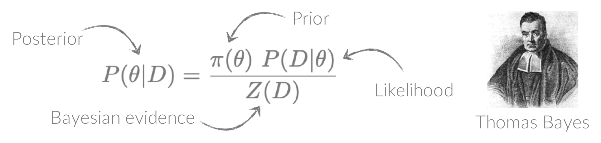
BXA connects PyXspec/Sherpa to nested sampling algorithms for Bayesian parameter estimation and model comparison with the Bayesian evidence.
Why use BXA?
Key strengths:
- Systematic fitting with minimal user input of initial parameters
- Efficient to systematically fit large datasets with many sources or compare many models
- Provides accurate parameter constraints, even for (very) low counts or for complex parameter spaces with strong degeneracies
Parameter space constraints in the (very) low count regime
BXA is capable of accurately estimating parameter confidence contours, even when no source counts are present. In this figure, a series of obscured accreting supermassive black hole (ak AGN)
spectra are simulated (left panel). The right panel then shows the BXA_derived confidence contours for intrinsic line of sight obscuring column density (log NH) vs. intrinsic
(i.e. unabsorbed) X-ray luminosity in the 2-10 keV band.
By simultaneously fitting the background and source spectra, BXA is able to derive a confidence contour for low count spectra even down to zero source counts (though the constraint is very poor,
as expected). The contour found makes sense, since an unobscured AGN (i.e. log NH ~ 20) should have been detected if it were very bright. This is why the upper left portion of
the contour plane is always ruled out.
No need for fine-tuning initial parameters
BXA does not require a single pre-defined position in the parameter space to start exploring. In this figure, a series of X-ray spectra are simulated at incrementally brighter fluxes. The right panel shows the confidence contour between two parameters in the simulations - black hole spin vs. the height of the X-ray emitting source above the black hole (assuming the lamp post geometry). Both parameters were assigned uninformative priors before fitting over a wide range of possible values. The size and shape of the confidence contours found are thus independent of any single initial parameter values.
Setup
⚠️ WARNING! ⚠️ BXA requires a working form of PyXspec and/or Sherpa.
Make sure either of these are installed before doing the exercises! Also note the exercises were written for BXA v4.0.5 - if some commands are not working as expected, check which version you are running.
For PyXspec users
First, install PyXspec:- Using PyXspec requires a source distribution of HEASoft. See install instructions here:
https://heasarc.gsfc.nasa.gov/docs/software/heasoft/
- Create a new conda environment:
$ conda create -n xspecbxa python=3.8 - Activate the new environment:
$ conda activate xspecbxa - Install BXA:
- With Anaconda:
$ conda install -c conda-forge bxa - With
pip(see warning below):
$ pip install requests corner astropy h5py cython scipy tqdm pandas
$ pip install bxa
- With Anaconda:
- Check PyXspec works:
$ python -c 'import xspec' - Check UltraNest works:
$ python -c 'import ultranest' - Check BXA works:
$ python -c 'import bxa.xspec as bxa'
For Sherpa users
- First, install CIAO and Sherpa in a conda environment:
https://cxc.cfa.harvard.edu/ciao/download/ - Once the install process has finished, check Sherpa works:
$ conda activate ciao-environment-name
$ sherpa
- Activate the environment:
$ conda activate ciao-environment-name - Install BXA:
- With Anaconda:
$ conda install -c conda-forge bxa - With
pip(see warning below):
$ pip install requests corner astropy h5py cython scipy tqdm pandas
$ pip install bxa
- With Anaconda:
- Check UltraNest works:
$ python -c 'import ultranest' - Check BXA works:
$ python -c 'import bxa.sherpa as bxa'
*⚠️ Warning!
Installing packages with
conda and pip can lead to package conflicts, such as:
ValueError: numpy.ndarray size changed, may indicate binary incompatibility. Expected 96 from C header, got 88 from PyObject
If this occurs, from inside your
conda environment use:
pip uninstall ultranest
conda install -c cond-forge ultranest
Useful links
Documentation
- Xspec & PyXspec documentation:
https://heasarc.gsfc.nasa.gov/xanadu/xspec/ - Sherpa reference for commands:
https://cxc.cfa.harvard.edu/sherpa/ahelp/sherpa4.html - UltraNest documentation:
https://johannesbuchner.github.io/UltraNest/readme.html - BXA documentation: https://johannesbuchner.github.io/BXA/index.html
Places to ask questions
- Xspec Facebook group:
https://www.facebook.com/groups/320119452570/?ref=share - Astrostatistics Facebook group:
https://www.facebook.com/groups/astro.r/?ref=share - Email!
Useful papers & documents
- X-ray Data Primer by CXC:
https://cxc.cfa.harvard.edu/cdo/xray_primer.pdf - Information on C-statistics (& modified C-statistics, aka W-stat) used in Xspec & Sherpa by Giacomo Vianello:
https://giacomov.github.io/Bias-in-profile-poisson-likelihood/ - Nested sampling review - Buchner (2021)
https://arxiv.org/abs/2101.09675 - PCA background - Simmonds et al., (2018, A&A)
https://ui.adsabs.harvard.edu/abs/2018A%26A...618A..66S/abstract - Simulation-based calibration of false-positive & false-negative rates - Baronchelli et al., (2018, MNRAS)
https://ui.adsabs.harvard.edu/abs/2018MNRAS.480.2377B/abstract - Bayesian Hierarchical Modelling with BXA:
- Baronchelli et al., (2020, MNRAS), Section A1
https://ui.adsabs.harvard.edu/abs/2020MNRAS.498.5284B/abstract - Kuraszkiewicz et al., (2021, ApJ), Section A1
https://ui.adsabs.harvard.edu/abs/2021ApJ...913..134K/abstract - Liu et al., (2021, arXiv), Section 3.7
https://ui.adsabs.harvard.edu/abs/2021arXiv210614522L/abstract
- Baronchelli et al., (2020, MNRAS), Section A1
Lectures & videos
- BiD4BEST Bayesian X-ray Spectral Analysis lectures by Johannes Buchner:
- Graduate-level course: Monte Carlo inference methods by Johannes Buchner:
- Bayesian inference workflow in astronomy and physics: https://youtu.be/D2P6xBR_2bQ
- Bayesian model comparison, curse of dimensionality, Importance Sampling: https://youtu.be/TfaGfFnsmW8
- Markov Chain Monte Carlo (MCMC) and diagnostics: https://youtu.be/YA6Ezh8CsrY
- Hamiltonian Monte Carlo (HMC) by Dr. Francesca Capel: https://youtu.be/nmHGyXsiaeI
- Nested Sampling from scratch - Practical Inference for Researchers in the Physical Sciences: https://youtu.be/baLFl_4ZwXw
- State-of-the art in nested sampling and MCMC: literature review: https://youtu.be/HFaqcB_H6MA
- BXA Tutorial at Chandra Data Science 2021 by Peter Boorman & Johannes Buchner:
- Interactive visualisation of the nested sampling algorithm in UltraNest:
https://johannesbuchner.github.io/UltraNest/method.html?highlight=demo#visualisation
Scripts
- Sherpa script for fitting obscured AGN with BXA:
https://github.com/JohannesBuchner/BXA/blob/master/examples/sherpa/xagnfitter.py - PosteriorStacker (for deriving sample distributions from individual source posterior distributions)
https://github.com/JohannesBuchner/PosteriorStacker - example_advanced_priors.py (shows how to include custom priors in BXA)
https://github.com/JohannesBuchner/BXA/blob/master/examples/xspec/example_advanced_priors.py
Citations
- Xspec (& PyXspec) citation - Arnaud et al., (1996; ASPC):
https://ui.adsabs.harvard.edu/abs/1996ASPC..101...17A/abstract - Sherpa citation - Freeman et al., (2001; SPIE):
https://ui.adsabs.harvard.edu/abs/2001SPIE.4477...76F/abstract In CIAO 4.13, you can use this command to get information on the latest release:sherpa> sherpa.citation('latest') - BXA citation - Buchner et al., (2014; A&A)
https://ui.adsabs.harvard.edu/abs/2014A%26A...564A.125B/abstract - UltraNest citation - Buchner (2021, JOSS)
https://arxiv.org/abs/2101.09604
- Load a spectrum and fit a model to it in Xspec, PyXspec and/or Sherpa
- Manually explore a parameter space and avoid local minima
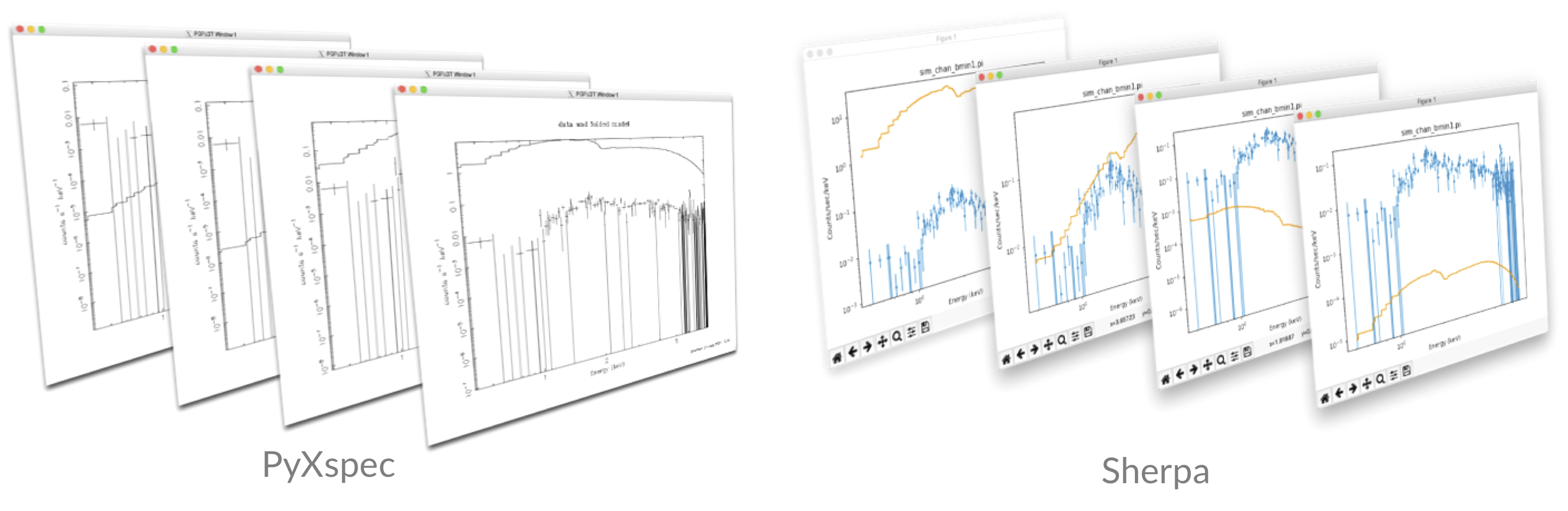
- Get to grips with plotting in Xspec, PyXspec and Sherpa
Getting started
If you don't have your own, download the following Chandra/ACIS spectral files from here. The zip file contains:- Source spectrum (binned with
ftgrouppha grouptype=bmin groupscale=1):sim_chan_bmin.pi - Response:
chan.rmf - Effective area:
chan.arf - Background spectrum:
sim_chan_bkg.pi
- For interactive mode:
- Xspec:
$ xspec - PyXspec:
$ ipython
from xspec import *
- Sherpa:
$ sherpa
- Xspec:
- For scripting:
- Xspec:
$ xspec - xspec_script.tclRemember to includeexitorquitat the end of the script! - PyXspec:
$ python3 pyxspec_script.py - Sherpa:
$ sherpa sherpa_script.py
- Xspec:
- Set the x-axis units (e.g., instrument channels or energy):
- Xspec:
setplot energy - PyXspec:
Plot.xAxis = "keV"# or "channel" - Sherpa:
set_analysis("ener")# or "chan"
- Xspec:
- Plot device (Xspec & PyXspec only):
- Xspec:
- Set the plot device:
cpd /xw
- Set the plot device:
- PyXspec:
- No plot device (useful to avoid plot window pop-ups):
Plot.device = "/null" - Set the plot device:
Plot.device = "/xw"
- No plot device (useful to avoid plot window pop-ups):
- Xspec:
- Load spectra:
- Ignore ineffective energies:
- Xspec:
setplot area/noarea:
For plots, divide the observed data by the response effective areasetplot add/noadd:
Show all additive model components in plotssetplot background/nobackground:
Automatically plot the background in the same plot as the sourcesetplot rebin X Y N:
Adjacent bins are combined in datasetNuntil either: (1) the significance of the combined bins is ≥ X σ or (2)Ybins have been combined. To undo on all datasets, usesetplot rebin 0 1 -1.setplot command range x 0.4 10.
To append any IPLOT commands to a list that is executed when the user typesplot .... For a full list of available commands, see:
- PyXspec (for command descriptions see above, for command documentation see here):
Plot.area=True/FalsePlot.add=True/FalsePlot.background=True/FalsePlot.setRebin(X, Y, N)Plot.addCommand("range x 0.4 10.")
- Xspec (note you can try
counts/data/lcountsin place ofldata):
setplot rebin 2 1000 -1
plot ldata
- PyXspec (note you can try
"counts"/"data"/"lcounts"in place of"ldata"):
Plot.setRebin(2, 1000) Plot("ldata") - Sherpa (note you can try
"counts"in place of"rate"):
group_snr(1, 2.)
subtract(1)
set_analysis(1, "ener", "rate")
plot_data(xlog=True, ylog=True)
Interactive PLT (Xspec only)
In Xspec, you can either use plot or iplot to produce plots. plot will make the plot and return the user to the Xspec prompt, whereas iplot starts the interactive plotting interface which can be used to edit a plot.
You can always view the full list of PLT commands being run by Xspec if you increase the verbosity to
chatter 25 before typing iplot. This is useful for determining the plotting element numbers for different colours, etc. Here are some basic commands for using the interactive PLT interface:
LAB title text: Change the title of the plot to "text"time off: Remove the time label in the bottom right of the plotCS N: Change the character size for text on the plot (values of 0-5 are allowed, 1 is default)viewport xlo ylo xhi yhi: Change the location of the plot in the plotting windowLAB y ylabel: Change the y axis labelLAB x xlabel: Change the x axis labelCOL 0 on 1..2: Change the colour of elements 1..2 to 0 (i.e. black - for all available colours, see Fig. 5.1 here)LW 5 on 1..2: Change the line width of elements 1-2 to 5 (values can be ≥ 1)LAB 5 POS x y "This text is... \fiITALIC\fn NORMAL\uSUPERSCRIPT\d\dSUBSCRIPT": create a text label.- Greek alphabet in order (use
\Gfor capitals):
\ga \gb \gg \gd \ge \gz \gy \gh \gi \gk \gl \gm \gn \gc, \go, \gp, \gr \gs \gt \gu \gf \gx \gq \gw
- Greek alphabet in order (use
LAB 5 COL 4 CS 1.4: Change the colour of label 5 to 4 (i.e. blue) and change the character size to 1.4
plot. To interact with this list of commands:
setplot command ...: Type this followed by any interactivePLTcommand to append the command to the listsetplot list: Show the currently appended plot commandssetplot delete all: Remove all plot commands from the list
wdata filename.dat inside interactive PLT (or use setplot command wdata filename.dat with Xspec plot) to save everything being plotted by Xspec to filename.dat (make sure to keep track of the order of the columns!). This file can then be read in with e.g., pandas to plot in Python.
Saving the data to be plotted by yourself can be done with the following:
- Xspec:
setplot rebin 2 1000 -1
setplot command wdata ldata_plot.dat
plot ldata
exit
Then the data can be read in to e.g.,pandaswith:import pandas as pd df = pd.read_csv("ldata_plot.dat", skiprows=3, delim_whitespace=True, names=["EkeV", "EkeV_err", "data", "data_err"]) - PyXspec:
import pandas as pd Plot.setRebin(2, 1000) EkeV = Plot.x() EkeV_err = Plot.xErr() data = Plot.y() data_err = Plot.yErr() df = pd.DataFrame(data={"EkeV": EkeV, "EkeV_err": EkeV_err, "data": data, "data_err": data_err}) - Sherpa:
import pandas as pd
group_snr(1, 2.)
subtract(1)
set_analysis(0, "ener", "rate")
srcdata = get_data_plot(1)
EkeV = srcdata.x
EkeV_err = srcdata.xerr
data = srcdata.y
data_err = srcdata.yerr
df = pd.DataFrame(data={"EkeV": EkeV, "EkeV_err": EkeV_err, "data": data, "data_err": data_err})
import matplotlib.pyplot as plt
fig, ax = plt.subplots()
err_kwargs = {}
err_kwargs["fmt"] = "o"
err_kwargs["label"] = "Folded data"
err_kwargs["mec"] = "royalblue"
err_kwargs["ecolor"] = "royalblue"
err_kwargs["mfc"] = "white"
err_kwargs["markersize"] = 6.
err_kwargs["markeredgewidth"] = 1.
err_kwargs["linewidth"] = 1.
err_kwargs["capthick"] = 0.
err_kwargs["capsize"] = 0.
err_kwargs["zorder"] = -1.
ax.errorbar(EkeV, data, xerr=EkeV_err, yerr=data_err, **err_kwargs)
ax.set_xscale("log")
ax.set_yscale("log")
plt.show()
fig.savefig("folded_data.png")
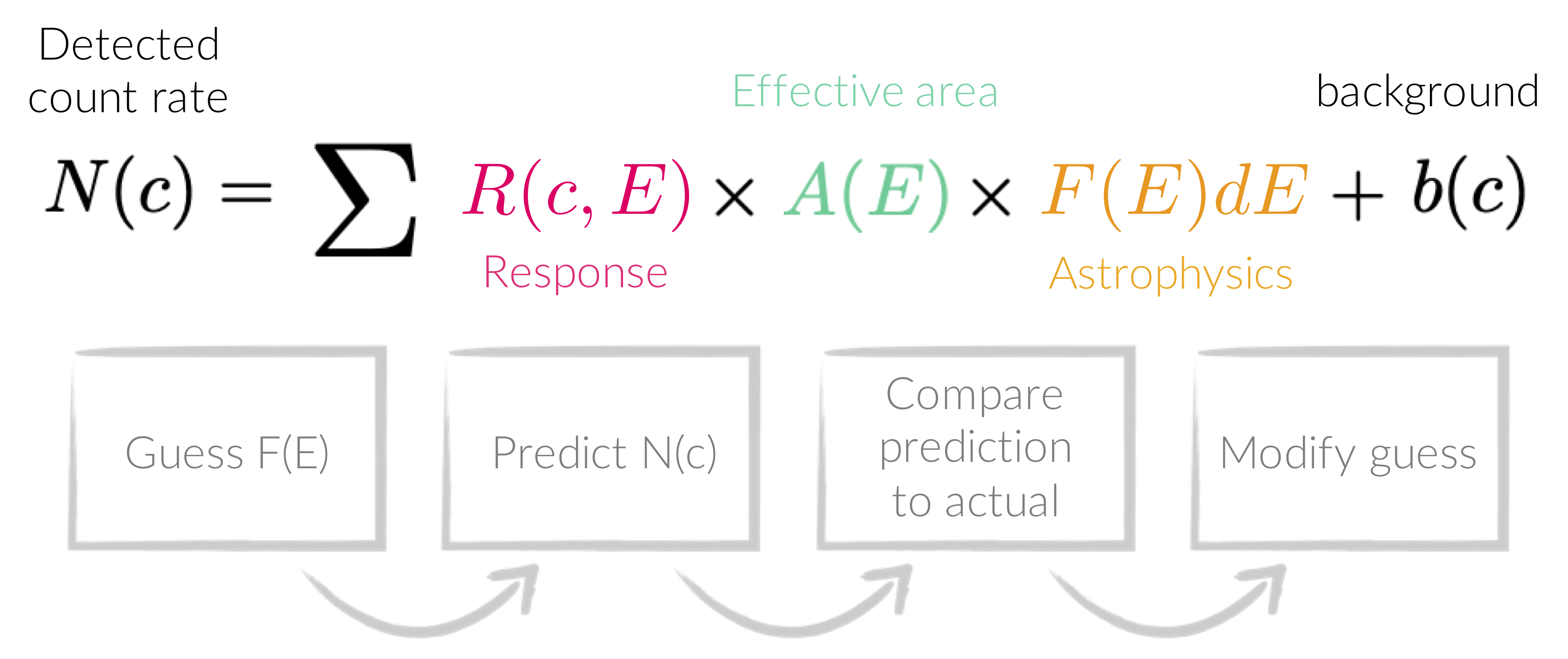
plot ldata in Xspec is not the true spectrum,
but a form of the true data that has been folded with all the effects arising from detecting the source.
This is why fitting is done with forward-folding.
Forward-folding is the process creating a model from some parameters, and then convolving it with the detector response and effective area. The convolved version of the model is then compared with the convolved data by some statistical measure, and is repeated until the parameters are optimised according to the statistical measure.
- Set the fit statistic (here we use modified Poisson statistics, which are appropriate in relatively low counts - see figure below):
- Xspec:
set stat cstat - PyXspec:
Fit.statMethod = "cstat" - Sherpa:
set_stat("wstat")
- Xspec:
- (Optional) turn off the interruption whilst fitting (Xspec & PyXspec only):
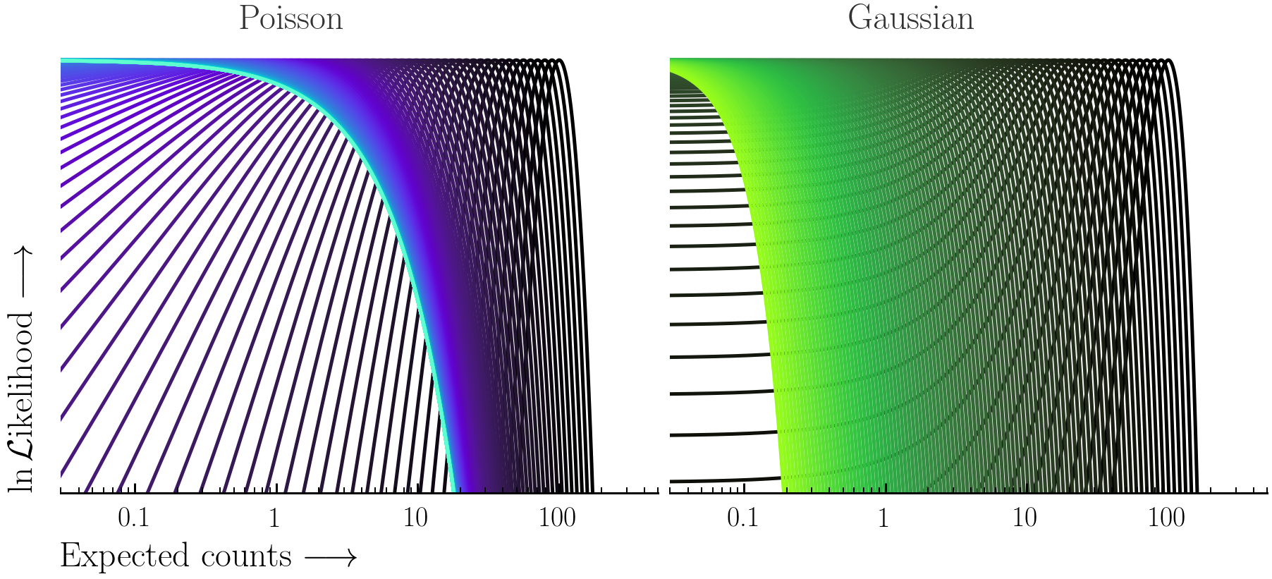
Here the Poisson and Gaussian statistics only become comparable in the high-count regime.
powerlaw model and set the model parameter values:
- Create the model:
- Xspec:
model powerlaw - PyXspec:
mymod = Model("powerlaw") - Sherpa:
mymod = xspowerlaw.mypow
set_source(1, mymod)
xsis used to indicate Xspec models, and get_default_id() can be used to show the id that is used if an id is not specified
- Xspec:
- Set the parameter values:
Note the
min,maxparameter bounds are used in the BXA priors and should be set to reasonable values.- Xspec:
newpar 1 1.9, 0.1, -1., -1., 4., 4.
newpar 2 1.e-3, 0.1, 1.e-8, 1.e-8, 1., 1.
- PyXspec:
mymod.powerlaw.PhoIndex.values = (1.9, 0.1, -1., -1., 4., 4.)
mymod.powerlaw.norm.values = (1.e-3, 0.1, 1.e-8, 1.e-8, 1., 1.)
Or:
AllModels(1)(1).values = 1.9, 0.1, -1., -1., 4., 4.
AllModels(1)(2).values = 1.e-3, 0.1, 1.e-8, 1.e-8, 1., 1.
- Xspec:
- Sherpa:
set_par(mypow.phoindex, val=1.9, min=-1., max=4.)
set_par(mypow.norm, val=1.e-3, min=1.e-8, max=1.)
- Xspec:
plot ldata del
fit
- PyXspec:
Plot("ldata del") Fit.perform() - Sherpa (note if you subtracted the data previously with
subtract, you need to rununsubtractif fitting withwstatorcstat):
plot_fit(xlog=True, ylog=True)
fit()
Beware of local minima!
Depending on where you start your fit, the Levenberg-Marquadt algorithm may struggle to find the global minimum (i.e. the true best-fit).In this example, both plots show an example progression for a fit with the Levenberg-Marquadt algorithm in Xspec. The final fit in the left panel is the global minimum, whereas the right hand plot is a local minimum. Local minima can be quite hard to identify visually and even masquerade as a very good fit. A quick way to initially check is to look for physically-unrealistic parameter values from a fit. The more thorough way to combat this issue whilst using Levenberg-Marquadt is to try to explore the parameter space more fully - e.g., with
steppar in Xspec/PyXspec or by manually starting the fit from different initial parameter values.
Have you found the best-fit parameter values for your
powerlaw fit? Try starting the parameters at different initial values before fitting to check.
Plotting a model with data
When plotting a model with data, there are a few options inside Xspec, PyXspec and Sherpa:- Folded units:
See the commands from Exercise 0.1 - Unfolded units:
Note that plotting in unfolded units is useful to see the possible unconvolved spectrum, but this is model dependent. Changing the model will change the plot.- Xspec:
plot ufspecplot eufspecplot eeufspec
- PyXspec:
Plot("ufspec")Plot("eufspec")Plot("eeufspec")
Note the model y-axis values can be accessed after running the
Plot(...)command with e.g.,mod_data = Plot.model(). - Sherpa:
See Sherpa thread here.
- Xspec:
- Residuals:
- Xspec:
- PyXspec (see equivalent descriptions above):
Plot("residuals")
Plot("ratio")
Plot("delchi")
plot_fit_resid(1)
Plot the data and folded model together with the residuals.plot_fit_ratio(1)
Plot the data and folded model together with the ratio of model to data.plot_fit_delchi(1)
Plot the data and folded model together with the residuals.
- Xspec:
steppar log/nolog parno1 lowerbound1 upperbound1 nsteps log/nolog parno2 lowerbound2 upperbound2 nsteps
plot cont
- PyXspec:
Fit.steppar("log/nolog parno1 lowerbound1 upperbound1 nsteps log/nolog parno2 lowerbound2 upperbound2 nsteps")
Plot("cont")
Note: you will have to choose the - Sherpa:
See Region Projection in this excellent Sherpa guide.
lowerbound and upperbound in steppar to encompass the parameter values.
Key objectives:
- Fit a spectrum with BXA in Sherpa and/or PyXspec
- Use Bayes factors to perform model comparison
- Visualise the confidence ranges on each parameter
To start with, make sure you import the relevant packages:
- PyXspec:
from xspec import *
import bxa.xspec as bxa
- Sherpa:
import bxa.sherpa as bxa
Exercise 1.1 - prior predictive checks
Prior predictive checks are useful to see if the priors chosen can lead to realistic model realisations.- PyXspec:
bxa.create_uniform_prior_for(model, param)
bxa.create_loguniform_prior_for(model, param)
bxa.create_gaussian_prior_for(model, param, mean, std)
- Sherpa:
bxa.create_uniform_prior_for(param)
bxa.create_loguniform_prior_for(param)
bxa.create_gaussian_prior_for(param, mean, std)
- Set the parameter priors for the
powerlawmodel (notenormvaries over many orders of magnitude, andPhoIndexcan be assigned a uniform prior for now):- PyXspec:
prior1 = bxa.create_uniform_prior_for(mymod, mymod.powerlaw.PhoIndex)
prior2 = bxa.create_loguniform_prior_for(mymod, mymod.powerlaw.norm)
- Sherpa:
prior1 = bxa.create_uniform_prior_for(mymod.PhoIndex)
prior2 = bxa.create_loguniform_prior_for(mymod.norm)
- PyXspec:
- A note on log parameters (Sherpa only):
Using a loguniform prior may not give the posterior values of that parameter in log units in Sherpa.
Instead, the
Parametermodule can convert a parameter to log units, and then one can use a uniform prior for that parameter. E.g.:from sherpa.models.parameter import Parameter logpar = Parameter(modelname, parname, value, min, max, hard_min, hard_max) mymod.norm = 10**logpar
Note the parameter will only be valid for working in BXA. If you want to define a log parameter and use this with a standard Sherpa fit, the log parameter must appear in the model expression.
- Create a solver:
- PyXspec:
solver = bxa.BXASolver(transformations=[prior1, prior2], outputfiles_basename="powerlaw_pyxspec") - Sherpa:
solver = bxa.BXASolver(prior=bxa.create_prior_function([prior1, prior2]),
                       parameters=[param1, param2],
                       outputfiles_basename="powerlaw_sherpa")
outputfiles_basenameis unique if running PyXspec and Sherpa in the same directory.- (For Sherpa) the priors are in the same order for the
priorandparametersattributes.
- PyXspec:
- Perform prior predictive checks:
- Generate random samples of prior parameter values (remember to
import numpy!):- PyXspec:
values = solver.prior_function(numpy.random.uniform(size=len(solver.paramnames))) - Sherpa:
values = solver.prior_transform(numpy.random.uniform(size=len(solver.paramnames)))
- PyXspec:
- Set the parameters to these values:
- PyXspec:
from bxa.xspec.solver import set_parameters
set_parameters(transformations=solver.transformations,values=values)
- Sherpa:
for i, p in enumerate(solver.parameters): p.val = values[i]
- PyXspec:
- Plot the resulting prior model samples (with the data to help guide the eye):
- Generate random samples of prior parameter values (remember to
- Produce 10 realisations of the model priors. Are the model ranges covered by the priors physically-acceptable?
- First fit the model using Levenberg-Marquadt included in Xspec & Sherpa:
- Is the fit good? How can you tell? What does changing the parameters by a small amount do?
- Next perform the fit with BXA (note this does not require fitting with Levenberg-Marquadt first):
(Note the hyperlinks are different).
resultscontains the posterior samples (results["samples"]) for each parameter and the Bayesian evidence (results["logZ"],results["logZerr"]). These quantities should also be printed to the screen after the fit is completed. To understand more about the information UltraNest prints to the screen during and after a fit, see here. - Examine the best-fit values and uncertainties from the posterior samples. This can be done with
pandas(may require installing with e.g.,conda install pandasbut see warning at the end of Setup):import pandas as pd df = pd.DataFrame(data=results["samples"], columns=solver.paramnames) df.head()
- How do the best-fits and confidence ranges compare with using nested sampling vs. Levenberg-Marquadt?
Exercise 1.3 - fit and compare multiple models
Here we use the Bayesian evidence to perform model comparison with Bayes factors.- Note to use
TBabs, one should set the abundances to those from Wilms, Allen & McCray (2000):- PyXspec:
Xset.abund = "wilm" - Sherpa:
set_xsabund("wilm")
- PyXspec:
- Using your previous code, fit the following additional 2 models to the data with BXA (don't forget to give unique
outputfiles_basenamevalues!):- Absorbed powerlaw:
For
nh, you can assumedelta = 0.1,min = 1.e-2,bottom = 1.e-2,top = 5.e2,max = 5.e2.- PyXspec:
TBabs * powerlaw - Sherpa:
xstbabs * xspowerlaw
- PyXspec:
- Absorbed powerlaw + Gaussian emission line (assume the emission line for this source is known to have line centroid energy
LineE= 6.3 ± 0.15 keV, and that the line is narrow with fixed widthSigma= 1.e-3 keV):- PyXspec (note to fix a parameter, you can set
delta = -1):TBabs * powerlaw + gaussian - Sherpa:
xstbabs * xspowerlaw + xsgaussian
- PyXspec (note to fix a parameter, you can set
- Absorbed powerlaw:
For
- Copy the model_compare.py script to your working directory to perform Bayesian evidence model comparison
- Run the script:
$ python3 model_compare.py outputfiles_basename1/ outputfiles_basename2/ outputfiles_basename3/ - Compute the Akaike Information Criterion (AIC) (given by
AIC = 2×nfree+Cstat ≡ 2×nfree-2×log(Likelihood), wherenfreeis the number of free fit parameters) for each model in python:import json basenames = [outputfiles_basename1, outputfiles_basename2, outputfiles_basename3] loglikes = dict([(f, json.load(open(f + "/info/results.json"))["maximum_likelihood"]["logl"]) for f in basenames]) nfree = dict([(f, len(json.load(open(f + "/info/results.json"))["paramnames"])) for f in basenames]) aic = dict([(basename, (2. * nfree[basename] - 2. * loglike)) for basename, loglike in loglikes.items()])
- Which model best explains the data? Why?
- Try adding a new additive
apeccomponent to the model:
- PyXspec:
mod4 = Model("TBabs * powerlaw + gaussian + apec") ... mod4.apec.kT.values = 0.8, 0.01, 1.e-2, 1.e-2, 5., 5. mod4.apec.Abundanc.values = 1., -1 mod4.apec.Redshift.values = 0., -1 mod4.apec.norm.values = 1.e-4, 0.1, 1.e-10, 1.e-10, 1.e-1, 1.e-1 - Sherpa:
xstbabs.tbabs * xspowerlaw.powerlaw + xsgaussian.gaussian + xsapec.apec
...
set_par(apec.kt, val=0.8, min=1.e-2, max=5.)
set_par(apec.abundanc, val=1., frozen=True)
set_par(apec.redshift, val=0., frozen=True)
set_par(apec.norm, val=1.e-4, min=1.e-10, max=1.e-1)
- PyXspec:
- How does the Bayesian Evidence from fitting the new
apecmodel to the data compare to the previous models?
Exercise 1.4 - error propagation
By generating quantities directly from the posterior samples, we propagate the uncertainties and conserve any structure (e.g., degeneracies, multiple modes).- The equivalent width (
EWbelow) of an emission line is defined as the flux in the line divided by the flux of the continuum at the line energy (see the Xspec documentation for more information). - For the model we have used, the equivalent width of the emission line relative to the intrinsic (i.e. unabsorbed) powerlaw continuum is (in terms of the parameters defined):
- PyXspec:
solver3.set_paramnames(["log(nH)", "mypow.phoindex", "mypow.lognorm", "line.linee", "line.lognorm"])
df = pd.DataFrame(data = results3["samples"], columns = solver3.paramnames)
df.loc[:, "EW"] = (10**df["line.lognorm"] / 10**df["mypow.lognorm"]) * df["line.linee"] ** df["mypow.phoindex"]
- Sherpa:
df = pd.DataFrame(data = results3["samples"], columns = solver3.paramnames)
df.loc[:, "EW"] = (df["line.norm"] / df["mypow.norm"]) * df["line.linee"] ** df["mypow.phoindex"]
- PyXspec:
- Use the
results["samples"]to derive the posterior distribution on equivalent width for the emission line component. If using pandas:import corner figure = corner.corner(df, labels = df.columns, quantiles = [0.16, 0.5, 0.84], show_titles = True)
- Is the equivalent width degenerate with any other parameters? Why or why not?
- First, examine the corner and trace plots that BXA produces (located in
outputfiles_basename/plots/). What do these plots show? - Are there any parameter degeneracies? Why or why not?
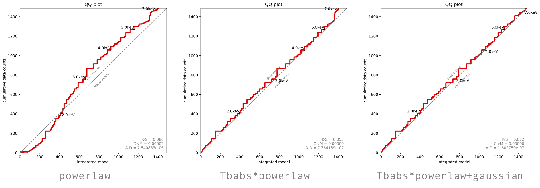
- Create a Quantile-Quantile (also here for a more general explanation) plot for your fits:
- PyXspec (produces plot):
Warning: if you have used
Plot.setRebin(), you should undo this before usingbxa.qqwith e.g.,Plot.setRebin(0., 1.)(or restart without runningPlot.setRebin())
import matplotlib.pyplot as plt
print("creating quantile-quantile plot ...")
plt.figure(figsize=(7,7))
with bxa.XSilence():
    solver.set_best_fit()
    bxa.qq.qq(prefix=outputfiles_basename, markers=5, annotate=True)
print("saving plot...")
plt.savefig(outputfiles_basename + "qq_model_deviations.pdf", bbox_inches="tight")
plt.close()
- Sherpa (produces file that needs to be plotted separately):
from bxa.sherpa.qq import qq_export
bxa.qq.qq_export(1, bkg=False, outfile=outputfiles_basename + "_qq", elow=0.2, ehigh=10)
- PyXspec (produces plot):
Warning: if you have used
- What does the
powerlawmodel Q-Q plot show? Is this model lacking any components? - (PyXspec only) Produce a plot of posterior model spectra (convolved and unconvolved) using the code in the example_simplest.py script included in BXA. Which energies is the model best-constrained over?
Exercise 1.6 - fitting multiple datasets simultaneously with BXA
Sometimes it is advantageous to fit multiple spectra for the same source simultaneously with e.g., a cross-calibration constant to account for instrumental differences in the separate spectra.
- Source spectrum (
sim_nuA_bmin1.pi) & background spectrum (sim_nuA_bkg.pi) here. - Response (
nustar.rmf) and effective area (point_30arcsecRad_1arcminOA.arf) files from the Point source simulation files (distributed by the NuSTAR team, more info here).
- First, include a cross-calibration constant in your model between the Chandra and NuSTAR datasets:
- PyXspec:
s = AllData("1:1 sim_nuA_bmin1.pi 2:2 sim_chan_bmin1.pi")
AllData.ignore("1:0.-3. 78.-** 2:0.-0.5 8.-**")
mymod = Model("constant * powerlaw")
AllModels(1)(1).values = (1., -0.01)
AllModels(2)(1).values = (1., 0.01, 0.01, 0.01, 10., 10.)
- Sherpa:
load_pha(1, "sim_nuA_bmin1.pi")
ignore_id(1, "0.:3.,78.:")
load_pha(2, "sim_chan_bmin1.pi")
ignore_id(2, "0.:0.5,8.:")
mymod = xspowerlaw.mypow
mymod1 = xsconstant("xcal1") * mymod
set_par(xcal1.factor, val=1, frozen=True)
mymod2 = xsconstant("xcal2") * mymod
set_par(xcal2.factor, val=1, min = 1.e-2, max = 1.e2)
set_source(1, mymod1)
set_source(2, mymod2)
- PyXspec:
- Fit the new model with BXA and derive a posterior confidence range on the cross-calibration constant:
- PyXspec:
prior1 = bxa.create_gaussian_prior_for(mymod, mymod.powerlaw.PhoIndex, 1.9, 0.15)
prior2 = bxa.create_loguniform_prior_for(mymod, mymod.powerlaw.norm)
transformations = [prior1, prior2]
transformations.append(bxa.create_loguniform_prior_for(AllModels(2), AllModels(2).constant.factor))
solver = bxa.BXASolver(transformations=transformations, outputfiles_basename="xcal_pl_pyxspec")
results = solver.run(resume=True)
- Sherpa:
prior1 = bxa.create_gaussian_prior_for(mymod, mymod.powerlaw.PhoIndex, 1.9, 0.15)
prior2 = bxa.create_loguniform_prior_for(mymod, mymod.powerlaw.norm)
priors = [prior1, prior2]
priors.append(bxa.create_loguniform_prior_for(xcal2))
parameters.append(xcal2)
solver = bxa.BXASolver(prior=bxa.create_prior_function([prior1, prior2, ...]), parameters=[param1, param2, ...], outputfiles_basename="xcal_pl_sherpa")
results = solver.run(resume=True)
mod4from the end of Exercise 1.3, the fit may take a long time to complete (up to an hour). - PyXspec:
- How have the confidence ranges on all the parameters changed after including NuSTAR?
- How have the Bayes factors between different model fits changed? Why?
auto_background function in BXA, which provides a powerful way to implement background models in Sherpa, and simultaneously fit with a source model using BXA.
- Load the data, source model and priors as in Exercise 1.1 (make sure to also change the statistic from
wstattocstat!) - Load the automatic PCA background model (see Simmonds et al., 2018 for more information):
from bxa.sherpa.background.pca import auto_background
set_model(1, model)
convmodel = get_model(1)
bkg_model = auto_background(1)
set_full_model(1, convmodel + bkg_model*get_bkg_scale(1))
- Remember to include the zeroth order component from the PCA background model in the priors and parameters list so that BXA knows to vary it as a free parameter:
parameters += [bkg_model.pars[0]]
priors += [bxa.create_uniform_prior_for(bkg_model.pars[0])]
- Fit the source + background model with BXA
- Check the background fit (e.g., with
get_bkg_fit,get_bkg_fit_ratio,get_bkg_fit_resid). - Have the uncertainty ranges changed at all for the parameters? Why or why not?
- Combine individual posteriors to constrain a population
- Calibrate model selection thresholds with simulations
- Perform model verification to test the Goodness-of-Fit
- PyXspec (using
fakeit):mymod = Model("powerlaw") mymod.powerlaw.PhoIndex.values = (1.9, 0.01, -3., -3., 3., 3.) mymod.powerlaw.norm.values = (1.e-3, 0.01, 1.e-8, 1.e-8, 1., 1.) fakeit_kwargs = {} fakeit_kwargs["response"] = "chan.rmf" fakeit_kwargs["arf"] = "chan.arf" fakeit_kwargs["background"] = "sim_chan_bkg.pi" fakeit_kwargs["exposure"] = 30.e3 fakeit_kwargs["correction"] = "1." fakeit_kwargs["backExposure"] = 30.e3 fakeit_kwargs["fileName"] = "sim_chan.pi" AllData.fakeit(1, FakeitSettings(**fakeit_kwargs))
- Sherpa (using
fake_pha):mymod = xspowerlaw.mypow set_par(mymod.phoindex, val = 1.9, min = -3., max = 3.) set_par(mymod.norm, val = 1.e-3, min = 1.e-8, max = 1.) load_pha(1, "chan_src.pi") #loading pre-exising source spectrum with rmf, arf & bkg present set_source(1, mymod) fakepha_kwargs = {} fakepha_kwargs["rmf"] = get_rmf() fakepha_kwargs["arf"] = get_arf() fakepha_kwargs["bkg"] = get_bkg() fakepha_kwargs["exposure"] = 30.e3 fake_pha(1, **fakepha_kwargs) save_pha(1, "sim_chan.pi", clobber = True)
Exercise 2.1 - Bayesian Hierarchical Modelling introduction
Here we will combine several individual source posterior distributions to derive a sample distribution for the photon index .
- Install PosteriorStacker:
$ conda install -c conda-forge posteriorstacker
Alternatively, you can just download the script and use it in your directory. - To generate the posterior samples used in this exercise, download and run the following PyXspec (
$ python3 ex21_pyxspec.py) or Sherpa ($ sherpa ex21_sherpa.py) script. The script will generate 30 UltraNest output folders by:- Simulating NuSTAR spectra from an
absorbed powerlawmodel (see Exercise 1.3), withPhoIndexsampled from a Gaussian distribution 1.8 +/- 0.3. Note you will need the Point source simulation files distributed by the NuSTAR team to run the scripts (more info here). - Each spectrum will then be fit with BXA using non-informative priors for line-of-sight column density, powerlaw photon index and powerlaw normalisation.
- Simulating NuSTAR spectra from an
- The script may take some time (~ a few hours) to complete. Alternatively, you can download some pre-generated UltraNest folders using a similar model here.
- From inside the
ultranest_posteriorsdirectory, run:$ load_ultranest_outputs.py fitsim0/ fitsim1/ fitsim2/ fitsim3/ fitsim4/ fitsim5/ fitsim6/ ... \ --samples 1000 \ --parameter PhoIndex \ --out posterior_samples.txt
- The
posterior_samples.txtfile contains 1000 sampled rows of each posterior. - Important: if the posterior samples were obtained with a non-uniform prior, the posterior samples should first be resampled according to the inverse of the prior that was used.
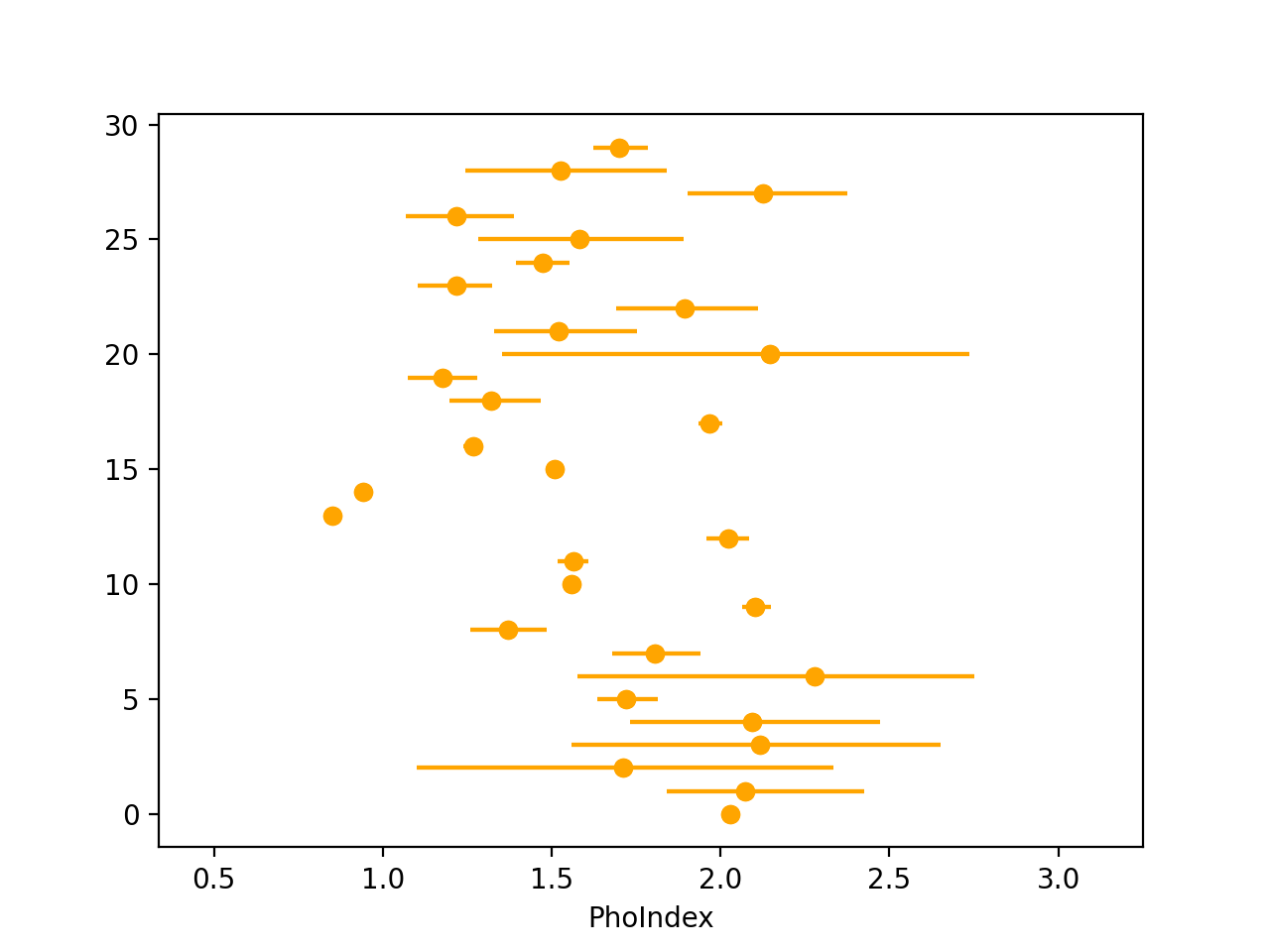
- Visualise the data by calculating the 16th, 50th & 84th quantiles of each posterior sample and plotting as an errorbar. E.g., in Python:
import numpy as np
import pandas as pd
quantiles = [16, 50, 84]
x = np.loadtxt("posterior_samples.txt")
q = np.percentile(x, quantiles, axis = 1)
df = pd.DataFrame(data = {"q%d" %(qvalue): q[i] for i, qvalue in enumerate(quantiles)})

import matplotlib.pyplot as plt
plt.xlabel("PhoIndex")
plt.errorbar(x=df["q50"], xerr=[df["q50"]-df["q16"], df["q84"]-df["q50"]], y=range(len(df)), marker="o", ls=" ", color="orange")
plt.xlim(df["q16"].min() - 0.5, df["q84"].max() + 0.5)
plt.show()
- Run PosteriorStacker:
$ posteriorstacker.py posterior_samples.txt 0.5 3. 10 --name="PhoIndex" - PosteriorStacker then fits two models for the parent sample distribution: a histogram model with each bin height as the free parameters (using a Dirichlet prior) and a Gaussian model with mean and sigma as the free parameters.
- Examine the
posteriorsamples.txt_out.pdffile. - What can you say about the distribution of
PhoIndex? What would happen if you acquired more posterior samples (i.e. by increasingpopulation_sizein the simulation scripts) and/or used higher signal-to-noise spectra to fit?
Exercise 2.2 - calibrating model comparison thresholds
Here we will estimate the false-positive and false-negative rates associated with selecting models via the Bayes Factors (logZmodel 1/Zmodel 2) & Δ fit-statistic for the models and data we are using. This helps us determine a good selection threshold to use for these model selection methods.
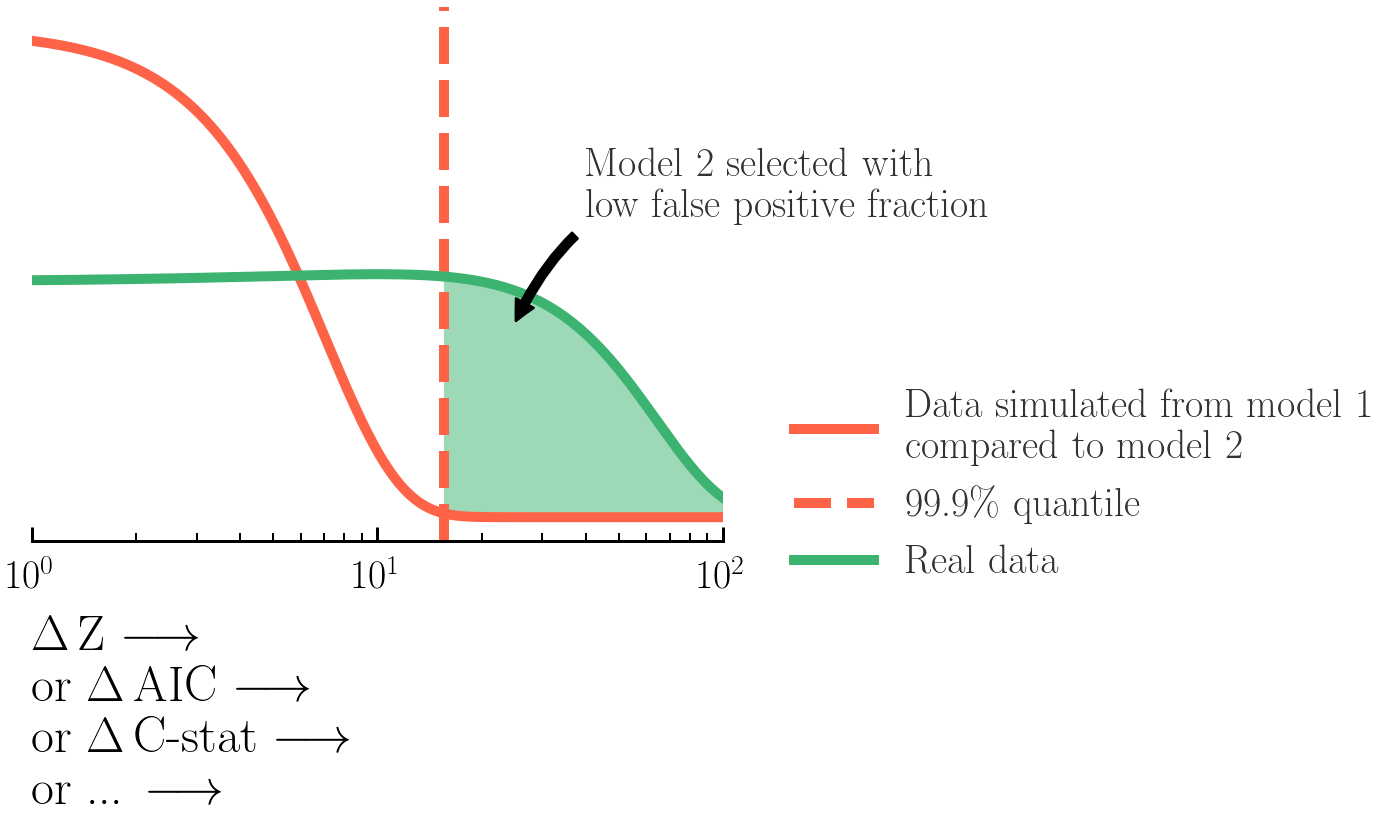
Here, you will estimate the false-negative and false-positive rates for model selection between the
powerlaw and absorbed powerlaw models from Exercises 1.2 and 1.3.
First, estimate the false-negative rate:
- Simulate 100 Chandra spectra from the
absorbed powerlaw(i.e. the more complex) best-fit model that you found in Exercise 1.3, with the original Chandra spectrum files. - Fit both the
powerlawandabsorbed powerlawmodels to each of the 100 simulated spectra with BXA. - For a series of different values of Δ logZ and Δ W-stat, calculate how many of the 100 model fits were correctly identified, and how many times the Bayes Factors did not make a decision (i.e. logZ1/Z2 < threshold).
- Use the same process to estimate an appropriate Δ W-stat threshold that will have a small false-negative rate.
- Repeat these step with a powerlaw normalisation 5× fainter than the best-fit.
- How does the false-negative rate vary with signal-to-noise in the source spectrum?
Then, estimate the false-positive rate:
- Simulate 100 Chandra spectra from the
powerlaw(i.e. the simplest) best-fit model that you found in Exercise 1.2, with the original Chandra spectrum files. - Fit both the
powerlawandabsorbed powerlawmodels to each of the 100 simulated spectra with BXA. - For a series of different values of Δ logZ and Δ W-stat, calculate how many of the 100 model fits selected a best-fit model that was not
powerlaw(i.e. a model was selected that was not the model being simulated). - Use the same process to estimate an appropriate Δ W-stat threshold that will have a small false-positive rate.
- Repeat these step with a powerlaw normalisation 5× fainter than the best-fit.
- How does the false-positive rate vary with signal-to-noise in the source spectrum?
- Repeat the process to estimate the false-negative and false-positive rates between
powerlawandabsorbed powerlaw + gaussianmodels. - Are the rates comparable? Why or why not?
Exercise 2.3 - posterior predictive checks
Model selection can only tell us how likely a model is relative to another. Here we will estimate the goodness-of-fit and test the ability of a given model to reproduce the nuances in the source spectrum data with Monte Carlo simulations.
- Load the BXA fit (with e.g.,
results = solver.run(resume=True)) for thepowerlawmodel from Exercise 1.2. - Note the best-fit C-statistic & degrees of freedom (dofs):
PyXspec:
stat = Fit.statistic
dof = Fit.dof
Sherpa:statinfo = get_stat_info() stat = statinfo[0].statval dof = statinfo[0].dof
- Perform many times:
- Simulate the best-fit model (make sure to use the same spectral files and exposure time as the original).
- Without re-fitting*, store the simulated C-statistic & dofs of the simulated data and model.
* It would be ideal to re-fit, but this can be inefficient and/or lead to incorrect results with a standard (i.e. Levenberg-Marquadt) fit in PyXspec and/or Sherpa due to local minima. Note also that to perform a Levenberg-Marquadt fit in Sherpa will require all free parameters, including specially-defined log parameters, to appear in the model expression.
- Plot the distribution of simulated C-statistic / dof values and compare to the real value. Is the fit acceptable?
- Now repeat the process with the
absorbed powerlaw + gaussianmodel. How does the goodness-of-fit for this model compare to thepowerlawmodel?
goodness command in Xspec. An alternative would be to run the same simulations, but plot the range of fluxes simulated for every spectral energy bin instead.
Exercise 2.4 (extension) - Bayesian Hierarchical Modelling continued
Now you have created a parent population for photon index using PosteriorStacker, this exercise will focus on the NH distribution.
The goal of this exercise is to estimate the uncertainty on each bin in a log NH distribution from a survey of 30 AGN.
For the AGN being simulated, we can assume:
- Every AGN follows the same baseline model:
model = TBabs[Gal] * TBabs[AGN] * powerlaw
Where:TBabs[Gal]is the absorbing column density arising from the Milky Way, assumed to be NH = 1020 cm-2 for every AGN.TBabs[AGN]is the absorbing column density at the source. This is the parameter we want to generate a population NH distribution from.powerlawis the intrinsic emission from the AGN, with photon index within 1.9 ± 0.1 and normalisation within 10-4 to 10-1 photons/keV/cm2/s at 1 keV.
Note this assumes that every AGN is at redshift zero.
- Every AGN has a column density NH in the range 1020 - 1025 cm-2. (Remember the units of NH in
TBabsis 1022 cm-2!) - Every AGN observation will be carried out by NuSTAR. Note the energy range for spectral analysis will be 3-78 keV, and you can assume observation exposures of 100 ks with no background present. Response (
nustar.rmf) and effective area (point_30arcsecRad_1arcminOA.arf) files can be found in the point source simulation files (distributed by the NuSTAR team, more info here). - The parent NH distribution follows this shape:
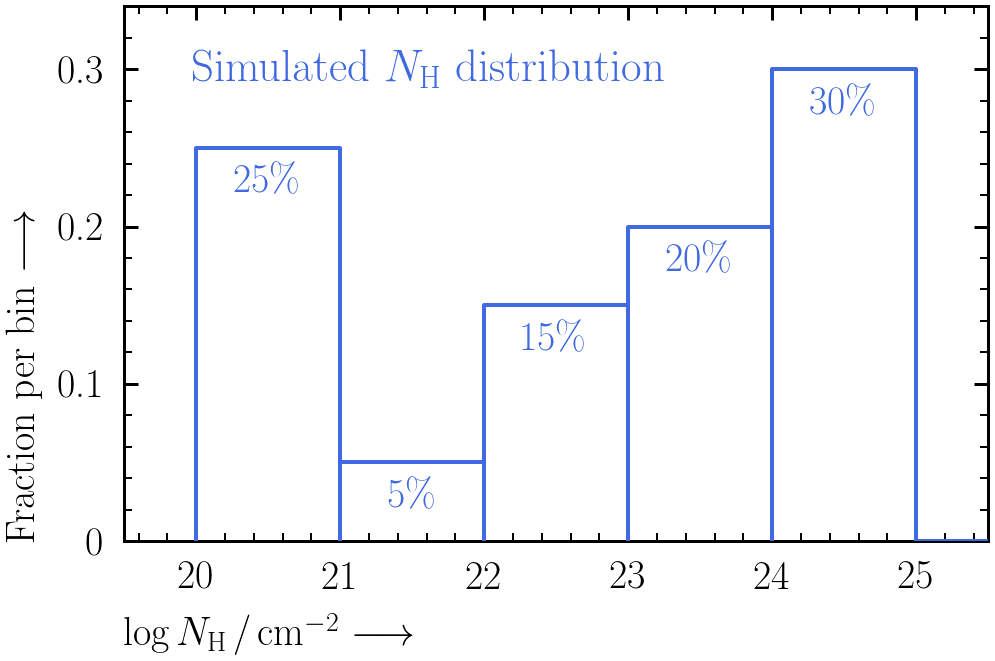
To generateNrandom log NH values from this distribution, you can use the following code:import scipy.interpolate import numpy as np np.random.seed(42) fractions = [0.25, 0.05, 0.15, 0.2, 0.3] bins = [20., 21., 22., 23., 24., 25.] cdf = np.append(0., np.cumsum(fractions) / np.sum(fractions)) interp_cdf = scipy.interpolate.interp1d(cdf, bins, bounds_error = False) rands = np.random.uniform(size = N) random_lognh_values = interp_cdf(rands)
- Simulate 30 AGN spectra from the model described in the assumptions above, each with a randomly generated log NH value.
- Re-fit each spectrum with BXA to generate log NH posteriors for each source.
- Combine the individual log NH posteriors with PosteriorStacker to estimate the NH distribution with the same bins as in the above plot.
- Estimate the fractions for each log NH bin from the histogram model
results["samples"], e.g.:
lo_hist = np.quantile(result["samples"], 0.16, axis = 0)
mid_hist = np.quantile(result["samples"], 0.5, axis = 0)
hi_hist = np.quantile(result["samples"], 0.84, axis = 0)
- Can your NH distribution constraints be improved? How could spectra below 3 keV help constrain the NH distribution?
-
To find the version of your bxa install:
import bxa, pkg_resources
print(pkg_resources.get_distribution("bxa").version)
- Speeding up BXA: For complex fits (e.g., multiple datasets simultaneously, many parameters, high signal-to-noise spectra, ...), the run time can be decreased with e.g.,:
- Parallelisation with MPI (Message Passing Interface):
mpiexec -np 4 python3 myscript.py - Arguments for
solver.run()
frac_remain=0.5sets the cut-off condition for the integration. A low value is optimal for finding peaks but higher values (e.g., 0.5) can be used if the posterior distribution is a relatively simple shape.max_num_improvement_loops=0sets the number of timesrun()will try to iteratively assess how many more samples are needed.speedspeed="safe"
Reactive Nested Sampler, recommended.speed="auto"
Step sampler with adaptive steps.speed=int
Step sampler with an integer number of steps. Faster, but the number of steps should be tested to ensure the log Z estimation is accurate.
- To see the other arguments of
run(), see here.
- If you're sure you want to, you can use BXA with chi-squared statistics:
bxa.BXASolver.allowed_stats.append("chi2") - You can create custom priors in BXA with
create_custom_prior_for()(example taken from example_advanced_prior.py): PyXspec:
def my_custom_prior(u):
    # prior distributions transform from 0:1 to the parameter range
    # here: a gaussian prior distribution, cut below 1/above 3
    x = scipy.stats.norm(1.9, 0.15).ppf(u)
    if x < 1.:
        x = 1
    if x > 3:
        x = 3
    return x
transformations = [bxa.create_custom_prior_for(model, parameter, my_custom_prior)]
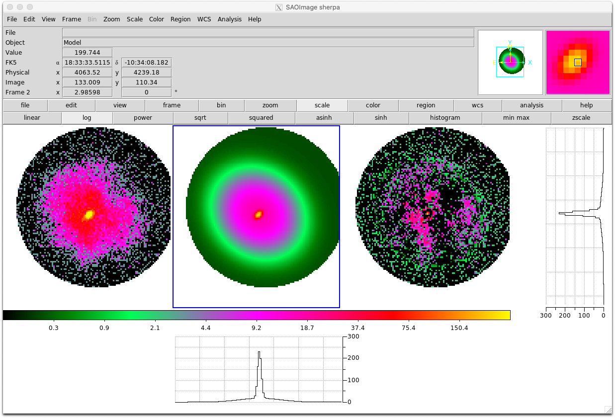
- You can use BXA with Sherpa to fit 2D models to images:
import bxa.sherpa as bxa
load_image("image.fits")
image_data()
set_coord("physical")
set_stat("cash")
model = gauss2d.g1 + gauss2d.g2 + const2d.bg
set_source(model)
set_par(g1.ampl, val = 20., min = 1., max = 1.e2)
...
parameters = [g1.ampl, ...]
priors = [bxa.create_loguniform_prior_for(g1.ampl), ...]
priorfunction = bxa.create_prior_function(priors)
solver = bxa.BXASolver(prior=priorfunction, parameters=parameters, outputfiles_basename = "fit2d_sherpa")
results = solver.run(resume=True)
image_data()
image_model(newframe=True)
image_resid(newframe=True)
Here is an example fit to the image used in this Sherpa tutorial for 2D fitting (left, middle and right panels show the image, best-fit model and residuals respectively):
- Parallelisation with MPI (Message Passing Interface):
- Using other sampling algorithms: Once the
solverobject has been created, you can acquire the log-Likelihood, parameter names and priors as follows:- PyXspec:
loglike = solver.log_likelihood
paramnames = solver.paramnames
prior = solver.prior_function
- Sherpa:
loglike = solver.log_likelihood
paramnames = solver.paramnames
prior = solver.prior_transform
These can then be passed to other sampling algorithms (including nested sampling) easily:- MCMC algorithms (e.g.,
emceeorzeus):
from autoemcee import ReactiveAffineInvariantSampler
sampler = ReactiveAffineInvariantSampler(paramnames, loglike, prior)
result = sampler.run()
- Laplace approximation, Importance Sampling:
from snowline import ReactiveImportanceSampler
sampler = ReactiveImportanceSampler(paramnames, loglike, transform)
result = sampler.run()
- Nested sampling:
from ultranest import ReactiveNestedSampler
sampler = ReactiveNestedSampler(paramnames, loglike, prior)
result = sampler.run()
- PyXspec:
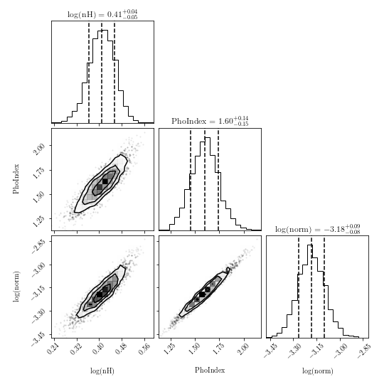
- Plotting contours:
There are a number of packages available to produce contour plots in Python. Here are a few examples, with some short code snippets to plot BXA posterior corner plots. Note the code snippets assume the posteriors are a pandas dataframe. To do this, you can type:
import pandas as pd outputfiles_basename = "example_basename" posterior = pd.read_csv("./%s/chains/equal_weighted_post.txt" %(example_basename), delim_whitespace=True)corner:
corner.readthedocs.io/en/latest/pages/quickstart.html
import corner fig = corner.corner(posterior.values, labels=posterior.columns, quantiles=[0.16, 0.5, 0.84], show_titles=True) fig.savefig("/path/to/your/corner.png")ChainConsumer:
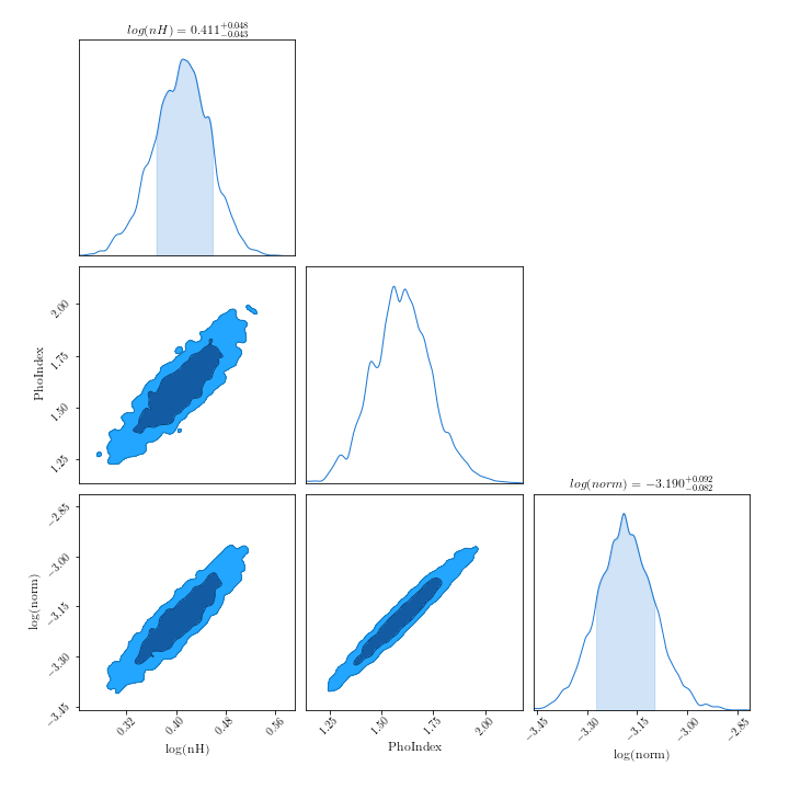
samreay.github.io/ChainConsumer/examples/plot_introduction.html
from chainconsumer import ChainConsumer c=ChainConsumer() c.add_chain(posterior.values, parameters = [r"%s" %(p) for p in posterior.columns]) fig=c.plotter.plot(figsize=(10, 10)) fig.savefig("/path/to/your/corner.png")GetDist:
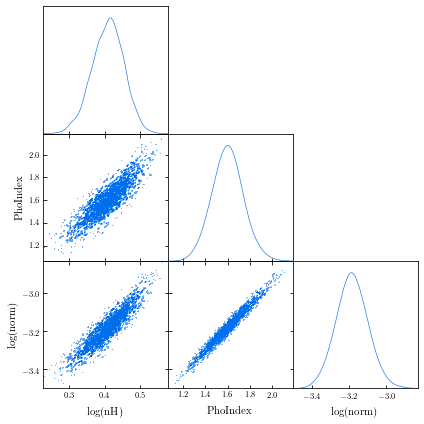
getdist.readthedocs.io/en/latest/plot_gallery.html
from getdist import plots, MCSamples
samples1 = MCSamples(samples=posterior.values, names=posterior.columns)
g = plots.get_subplot_plotter()
g.triangle_plot(samples1, filled=True)
g.export("/path/to/your/corner.png")
Note the confidence regions in 2D histograms are not the same as in 1D histograms. See this webpage from
corner for more information.